
Detmar STRAUB, David GEFEN, and Jan RECKER
Shortcut to Sections
- Section 1: Welcome and Disclaimers
- Section 2: What is Quantitative, Positivist Research
- Section 3: Philosophical Foundations
- Section 4: Fundamentals of QtPR
- Section 5: The General QtPR Research Approach
- Section 6: Practical Tips for Writing QtPR Papers
- Section 7: Glossary
- Section 8: Bibliography
Section 1. Welcome and Disclaimers
Welcome to the online resource on Quantitative, Positivist Research (QtPR) Methods in Information Systems (IS). This resource seeks to address the needs of quantitative, positivist researchers in IS research – in particular those just beginning to learn to use these methods. IS research is a field that is primarily concerned with socio-technical systems comprising individuals and collectives that deploy digital information and communication technology for tasks in business, private, or social settings. We are ourselves IS researchers but this does not mean that the advice is not useful to researchers in other fields.
This webpage is a continuation and extension of an earlier online resource on Quantitative Positivist Research that was originally created and maintained by Detmar STRAUB, David GEFEN, and Marie BOUDREAU. As the original online resource hosted at Georgia State University is no longer available, this online resource republishes the original material plus updates and additions to make what is hoped to be valuable information accessible to IS scholars. Given that the last update of that resource was 2004, we also felt it prudent to update the guidelines and information to the best of our knowledge and abilities. If readers are interested in the original version, they can refer to a book chapter (Straub et al., 2005) that contains much of the original material.
1.1 Objective of this Website
This resource is dedicated to exploring issues in the use of quantitative, positivist research methods in Information Systems (IS). We intend to provide basic information about the methods and techniques associated with QtPR and to offer the visitor references to other useful resources and to seminal works.
1.2 Feedback
Suggestions on how best to improve on the site are very welcome. Please contact us directly if you wish to make suggestions on how to improve the site. No faults in content or design should be attributed to any persons other than ourselves since we made all relevant decisions on these matters. You can contact the co-editors at: straubdetmar@gmail.com, gefend@drexel.edu, and jan.christof.recker@uni-hamburg.de.
1.3 How to Navigate this Resource
This resource is structured into eight sections. You can scroll down or else simply click above on the shortcuts to the sections that you wish to explore next.
1.4 Explanation for Self-Citations
One of the main reasons we were interested in maintaining this online resource is that we have already published a number of articles and books on the subject. We felt that we needed to cite our own works as readily as others to give readers as much information as possible at their fingertips.
1.5 What This Resource Does Not Cover
This website focuses on common, and some would call traditional approaches to QtPR within the IS community, such as survey or experimental research. There are many other types of quantitative research that we only gloss over here, and there are many alternative ways to analyze quantitative data beyond the approaches discussed here. This is not to suggest in any way that these methods, approaches, and tools are not invaluable to an IS researcher. Only that we focus here on those genres that have traditionally been quite common in our field and that we as editors of this resource feel comfortable in writing about.
One such example of a research method that is not covered in any detail here would be meta-analysis. Meta-analyses are extremely useful to scholars in well-established research streams because they can highlight what is fairly well known in a stream, what appears not to be well supported, and what needs to be further explored. Importantly, they can also serve to change directions in a field. There are numerous excellent works on this topic, including the book by Hedges and Olkin (1985), which still stands as a good starter text, especially for theoretical development.
1.6 How to Cite this Resource
You can cite this online resource as:
Straub, D. W., Gefen, D., Recker, J., “Quantitative Research in Information Systems,” Association for Information Systems (AISWorld) Section on IS Research, Methods, and Theories, last updated March 25, 2022, http://www.janrecker.com/quantitative-research-in-information-systems/.
The original online resource that was previously maintained by Detmar Straub, David Gefen, and Marie-Claude Boudreau remains citable as a book chapter: Straub, D.W., Gefen, D., & Boudreau, M-C. (2005). Quantitative Research. In D. Avison & J. Pries-Heje (Eds.), Research in Information Systems: A Handbook for Research Supervisors and Their Students (pp. 221-238). Elsevier.
Section 2: What is Quantitative, Positivist Research (QtPR)
2.1 Cornerstones of Quantitative, Positivist Research
QtPR is a set of methods and techniques that allows IS researchers to answer research questions about the interaction of humans and digital information and communication technologies within the sociotechnical systems of which they are comprised. There are two cornerstones in this approach to research.
The first cornerstone is an emphasis on quantitative data. QtPR describes a set of techniques to answer research questions with an emphasis on state-of-the-art analysis of quantitative data, that is, types of data whose value is measured in the form of numbers, with a unique numerical value associated with each data set. As the name suggests, quantitative methods tend to specialize in “quantities,” in the sense that numbers are used to represent values and levels of measured variables that are themselves intended to approximate theoretical constructs. Often, the presence of numeric data is so dominant in quantitative methods that people assume that advanced statistical tools, techniques, and packages to be an essential element of quantitative methods. While this is often true, quantitative methods do not necessarily involve statistical examination of numbers. Simply put, QtPR focus on how you can do research with an emphasis on quantitative data collected as scientific evidence. Sources of data are of less concern in identifying an approach as being QtPR than the fact that numbers about empirical observations lie at the core of the scientific evidence assembled. A QtPR researcher may, for example, use archival data, gather structured questionnaires, code interviews and web posts, or collect transactional data from electronic systems. In any case, the researcher is motivated by the numerical outputs and how to imbue them with meaning.
The second cornerstone is an emphasis on (post-) positivist philosophy. As will be explained in Section 3 below, it should be noted that “quantitative, positivist research” is really just shorthand for “quantitative, post-positivist research.” Without delving into many details at this point, positivist researchers generally assume that reality is objectively given, that it is independent of the observer (researcher) and their instruments, and that it can be discovered by a researcher and described by measurable properties. Interpretive researchers, on the other hand, start out with the assumption that access to reality (given or socially constructed) is only through social constructions such as language, consciousness, and shared meanings. While these views do clearly differ, researchers in both traditions also agree on several counts. For example, both positivist and interpretive researchers agree that theoretical constructs, or important notions such as causality, are social constructions (e.g., responses to a survey instrument).
2.2 Quantitative, Positivist Research for Theory-Generation versus Theory-Evaluation
What are theories? There is a vast literature discussing this question and we will not embark on any kind of exegesis on this topic. A repository of theories that have been used in information systems and many other social science theories can be found at: https://guides.lib.byu.edu/c.php?g=216417&p=1686139.
In simple terms, in QtPR it is often useful to understand theory as a lawlike statement that attributes causality to sets of variables, although other conceptions of theory do exist and are used in QtPR and other types of research (Gregor, 2006). One common working definition that is often used in QtPR research refers to theory as saying “what is, how, why, when, where, and what will be. [It provides] predictions and has both testable propositions and causal explanations (Gregor, 2006, p. 620).”
QtPR can be used both to generate new theory as well as to evaluate theory proposed elsewhere. In theory-generating research, QtPR researchers typically identify constructs, build operationalizations of these constructs through measurement variables, and then articulate relationships among the identified constructs (Im & Wang, 2007). In theory-evaluating research, QtPR researchers typically use collected data to test the relationships between constructs by estimating model parameters with a view to maintain good fit of the theory to the collected data.
Traditionally, QtPR has been dominant in this second genre, theory-evaluation, although there are many applications of QtPR for theory-generation as well (e.g., Im & Wang, 2007; Evermann & Tate, 2011). Historically however, QtPR has by and large followed a particular approach to scientific inquiry, called the hypothetico-deductive model of science (Figure 1).
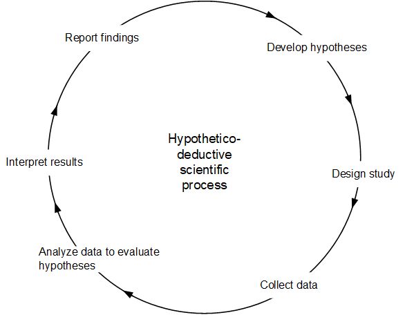
This model suggests that the underlying view that leads a scholar to conclude that QtPR can produce knowledge is that the world has an objective reality that can be captured and translated into models that imply testable hypotheses, usually in the form of statistical or other numerical analyses. In turns, a scientific theory is one that can be falsified through careful evaluation against a set of collected data.
The original inspiration for this approach to science came from the scientific epistemology of logical positivism during the 1920s and 1930s as developed by the Vienna Circle of Positivists, primarily Karl Popper,. This “pure” positivist attempt at viewing scientific exploration as a search for the Truth has been replaced in recent years with the recognition that ultimately all measurement is based on theory and hence capturing a truly “objective” observation is impossible (Coombs, 1976). Even the measurement of a purely physical attribute, such as temperature, depends on the theory of how materials expand in heat. Hence interpreting the readings of a thermometer cannot be regarded as a pure observation but itself as an instantiation of theory.
As suggested in Figure 1, at the heart of QtPR in this approach to theory-evaluation is the concept of deduction. Deduction is a form of logical reasoning that involves deriving arguments as logical consequences of a set of more general premises. It involves deducing a conclusion from a general premise (i.e., a known theory), to a specific instance (i.e., an observation). There are three main steps in deduction (Levallet et al. 2021):
- Testing internal consistency, i.e., verifying that there are no internal contradictions.
- Distinguishing between the logical basics of the theory and its empirical, testable, predictions.
- Empirical testing aimed at falsifying the theory with data. When the data do not contradict the hypothesized predictions of the theory, it is temporarily corroborated. The objective of this test is to falsify, not to verify, the predictions of the theory. Verifications can be found for almost any theory if one can pick and choose what to look at.
Whereas seeking to falsify theories is the idealistic and historical norm, in practice many scholars in IS and other social sciences are, in practice, seeking confirmation of their carefully argued theoretical models (Gray & Cooper, 2010; Burton-Jones et al., 2017). For example, QtPR scholars often specify what is called an alternative hypothesis rather than the null hypothesis (an expectation of no effect), that is, they typically formulate the expectation of a directional, signed effect of one variable on another. Doings so confers some analytical benefits (such as using a one-tailed statistical test rather than a two-tailed test), but the most likely reason for doing this is that confirmation, rather than disconfirmation of theories is a more common way of conducting QtPR in modern social sciences (Edwards & Berry, 2010; Mertens & Recker, 2020). In Popper’s falsification view, for example, one instance of disconfirmation disproves an entire theory, which is an extremely stringent standard. More information about the current state-of the-art follows later in section 3.2 below, which discusses Lakatos’ contributions to the philosophy of science.
In conclusion, recall that saying that QtPR tends to see the world as having an objective reality is not equivalent to saying that QtPR assumes that constructs and measures of these constructs are being or have been perfected over the years. In fact, Cook and Campbell (1979) make the point repeatedly that QtPR will always fall short of the mark of perfect representation. For this reason, they argue for a “critical-realist” perspective, positing that “causal relationships cannot be perceived with total accuracy by our imperfect sensory and intellective capacities” (p. 29). This is why we argue in more detail in Section 3 below that modern QtPR scientists have really adopted a post-positivist perspective.
2.3 What QtPR is Not
QtPR is not math analytical modeling, which typically depends on mathematical derivations and assumptions, sans data. This difference stresses that empirical data gathering or data exploration is an integral part of QtPR, as is the positivist philosophy that deals with problem-solving and the testing of the theories derived to test these understandings.
QtPR is also not design research, in which innovative IS artifacts are designed and evaluated as contributions to scientific knowledge. Models and prototypes are frequently the products of design research. In QtPR, models are also produced but most often causal models whereas design research stresses ontological models. Also, QtPR typically validates its findings through testing against empirical data whereas design research can also find acceptable validation of a new design through mathematical proofs of concept or through algorithmic analyses alone. Still, it should be noted that design researchers are increasingly using QtPR methods, specifically experimentation, to validate their models and prototypes so QtPR is also becoming a key tool in the arsenal of design science researchers.
QtPR is also not qualitative positivist research (QlPR) nor qualitative interpretive research. More information about qualitative research in both variants is available on an AIS-sponsored online resource. The simplest distinction between the two is that quantitative research focuses on numbers, and qualitative research focuses on text, most importantly text that captures records of what people have said, done, believed, or experienced about a particular phenomenon, topic, or event. Qualitative research emphasizes understanding of phenomena through direct observation, communication with participants, or analyses of texts, and at times stress contextual subjective accuracy over generality. What matters here is that qualitative research can be positivist (e.g., Yin, 2009; Clark, 1972; Glaser & Strauss, 1967) or interpretive (e.g., Walsham, 1995; Elden & Chisholm, 1993; Gasson, 2004). Without delving too deeply into the distinctions and their implications, one difference is that qualitative positive researchers generally assume that reality can be discovered to some extent by a researcher as well as described by measurable properties (which are social constructions) that are independent of the observer (researcher) and created instruments and instrumentation. Qualitative interpretive researchers start out with the assumption that access to reality (given or socially constructed) is only through social constructions such as language, consciousness, and shared meanings. Interpretive researchers generally attempt to understand phenomena through the meanings that people assign to them.
These nuances impact how quantitative or qualitative researchers conceive and use data, they impact how researchers analyze that data, and they impact the argumentation and rhetorical style of the research (Sarker et al., 2018). It does not imply that certain types of data (e.g., numerical data) is reserved for only one of the traditions. For example, QlPR scholars might interpret some quantitative data as do QtPR scholars. However, the analyses are typically different: QlPR might also use statistical techniques to analyze the data collected, but these would typically be descriptive statistics, t-tests of differences, or bivariate correlations, for example. More advanced statistical techniques are usually not favored, although of course, doing so is entirely possible (e.g., Gefen & Larsen, 2017).
Section 3. Philosophical Foundations
In what follows, we discuss at some length what have historically been the views about the philosophical foundations of science in general and QtPR in particular. We note that these are our own, short-handed descriptions of views that have been, and continue to be, debated at length in ongoing philosophy of science discourses. Readers interested primarily in the practical challenges of QtPR might want to skip this section. Also, readers with a more innate interest in the broader discussion of philosophy of science might want to consult the referenced texts and their cited texts directly.
3.1 A Brief Introduction to Positivism
QtPR researchers historically assumed that reality is objectively given and can be discovered by a researcher and described by measurable properties independent of the observer (researcher) and their instruments. This worldview is generally called positivism.
At the heart of positivism is Karl Popper’s dichotomous differentiation between “scientific” theories and “myth.” A scientific theory is a theory whose predictions can be empirically falsified, that is, shown to be wrong. Therefore, a scientific theory is by necessity a risky endeavor, i.e., it may be thrown out if not supported by the data. Einstein’s Theory of Relativity is a prime example, according to Popper, of a scientific theory. When Einstein proposed it, the theory may have ended up in the junk pile of history had its empirical tests not supported it, despite the enormous amount of work put into it and despite its mathematical appeal. The reason Einstein’s theory was accepted was because it was put to the test: Eddington’s eclipse observation in 1919 confirmed its predictions, predictions that were in contrast to what should have been seen according to Newtonian physics. Eddington’s eclipse observation was a make-or-break event for Einstein’s theory. The theory would have been discredited had the stars not appeared to move during the eclipse because of the Sun’s gravity. In contrast, according to Popper, is Freud’s theory of psychoanalysis which can never be disproven because the theory is sufficiently imprecise to allow for convenient “explanations” and the addition of ad hoc hypotheses to explain observations that contradict the theory. The ability to explain any observation as an apparent verification of psychoanalysis is no proof of the theory because it can never be proven wrong to those who believe in it. A scientific theory, in contrast to psychoanalysis, is one that can be empirically falsified. This is the Falsification Principle and the core of positivism. Basically, experience can show theories to be wrong, but can never prove them right. It is an underlying principle that theories can never be shown to be correct.
This demarcation of science from the myths of non-science also assumes that building a theory based on observation (through induction) does not make it scientific. Science, according to positivism, is about solving problems by unearthing truth. It is not about fitting theory to observations. That is why pure philosophical introspection is not really science either in the positivist view. Induction and introspection are important, but only as a highway toward creating a scientific theory. Central to understanding this principle is the recognition that there is no such thing as a pure observation. Every observation is based on some preexisting theory or understanding.
Furthermore, it is almost always possible to choose and select data that will support almost any theory if the researcher just looks for confirming examples. Accordingly, scientific theory, in the traditional positivist view, is about trying to falsify the predictions of the theory.
In theory, it is enough, in Popper’s way of thinking, for one observation that contradicts the prediction of a theory to falsify it and render it incorrect. Furthermore, even after being tested, a scientific theory is never verified because it can never be shown to be true, as some future observation may yet contradict it. Accordingly, a scientific theory is, at most, extensively corroborated, which can render it socially acceptable until proven otherwise. Of course, in reality, measurement is never perfect and is always based on theory. Hence, positivism differentiates between falsification as a principle, where one negating observation is all that is needed to cast out a theory, and its application in academic practice, where it is recognized that observations may themselves be erroneous and hence where more than one observation is usually needed to falsify a theory.
This notion that scientists can forgive instances of disproof as long as the bulk of the evidence still corroborates the base theory lies behind the general philosophical thinking of Imre Lakatos (1970). In Lakatos’ view, theories have a “hard core” of ideas, but are surrounded by evolving and changing supplemental collections of both hypotheses, methods, and tests – the “protective belt.” In this sense, his notion of theory was thus much more fungible than that of Popper.
In QtPR practice since World War II, moreover, social scientists have tended to seek out confirmation of a theoretical position rather than its disconfirmation, a la Popper. This is reflected in their dominant preference to describe not the null hypothesis of no effect but rather alternative hypotheses that posit certain associations or directions in sign. In other words, QtPR researchers are generally inclined to hypothesize that a certain set of antecedents predicts one or more outcomes, co-varying either positively or negatively. It needs to be noted that positing null hypotheses of no effect remains a convention in some disciplines; but generally speaking, QtPR practice favors stipulating certain directional effects and certain signs, expressed in hypotheses (Edwards & Berry, 2010). Overall, modern social scientists favor theorizing models with expressed causal linkages and predictions of correlational signs. Popper’s contribution to thought – specifically, that theories should be falsifiable – is still held in high esteem, but modern scientists are more skeptical that one conflicting case can disprove a whole theory, at least when gauged by which scholarly practices seem to be most prevalent.
3.2 From Positivism to Post-Positivism
We already noted above that “quantitative, positivist research” is really a shorthand for “quantitative, post-positivist research.” Whereas qualitative researchers sometimes take ownership of the concept of post-positivism, there is actually little quarrel among modern quantitative social scientists over the extent to which we can treat the realities of the world as somehow and truly “objective.” A brief history of the intellectual thought behind this may explain what is meant by this statement.
Flourishing for a brief period in the early 1900s, logical positivism, which argued that all natural laws could be reduced to the mathematics of logic, was one culmination of a deterministic positivism, but these ideas came out of a long tradition of thinking of the world as an objective reality best described by philosophical determinism. One could trace this lineage all the way back to Aristotle and his opposition to the “metaphysical” thought of Plato, who believed that the world as we see it has an underlying reality (forms) that cannot be objectively measured or determined. The only way to “see” that world, for Plato and Socrates, was to reason about it; hence, Plato’s philosophical dialecticism.
During more modern times, Henri de Saint-Simon (1760–1825), Pierre-Simon Laplace (1749–1827), Auguste Comte (1798–1857), and Émile Durkheim (1858–1917) were among a large group of intellectuals whose basic thinking was along the lines that science could uncover the “truths” of a difficult-to-see reality that is offered to us by the natural world. Science achieved this through the scientific method and through empiricism, which depended on measures that could pierce the veil of reality. With the advent of experimentalism especially in the 19th century and the discovery of many natural, physical elements (like hydrogen and oxygen) and natural properties like the speed of light, scientists came to believe that all natural laws could be explained deterministically, that is, at the 100% explained variance level. However, in 1927, German scientist Werner Heisenberg struck down this kind of thinking with his discovery of the uncertainty principle. This discovery, basically uncontended to this day, found that the underlying laws of nature (in Heisenberg’s case, the movement and position of atomic particles), were not perfectly predictable, that is to say, deterministic. They are stochastic. Ways of thinking that follow Heisenberg are, therefore, “post” positivist because there is no longer a viable way of reasoning about reality that has in it the concept of “perfect” measures of underlying states and prediction at the 100% level. These states can be individual socio-psychological states or collective states, such as those at the organizational or national level.
To illustrate this point, consider an example that shows why archival data can never be considered to be completely objective. Even the bottom line of financial statements is structured by human thinking. What is to be included in “revenues,” for example, is impacted by decisions about whether booked revenues can or should be coded as current period revenues. Accounting principles try to control this, but, as cases like Enron demonstrate, it is possible for reported revenues or earnings to be manipulated. In effect, researchers often need to make the assumption that the books, as audited, are accurate reflections of the firm’s financial health. Researchers who are permitted access to transactional data from, say, a firm like Amazon, are assuming, moreover, that the data they have been given is accurate, complete, and representative of a targeted population. But is it? Intermediaries may have decided on their own not to pull all the data the researcher requested, but only a subset. Their selection rules may then not be conveyed to the researcher who blithely assumes that their request had been fully honored. Finally, governmental data is certainly subject to imperfections, lower quality data that the researcher is her/himself unaware of. Adjustments to government unemployment data, for one small case, are made after the fact of the original reporting. Are these adjustments more or less accurate than the original figures? In the vast majority of cases, researchers are not privy to the process so that they could reasonably assess this. We might say that archival data might be “reasonably objective,” but it is not purely ”objective” By any stretch of the imagination. There is no such thing. All measures in social sciences, thus, are social constructions that can only approximate a true, underlying reality.
Our development and assessment of measures and measurements (Section 5) is another simple reflection of this line of thought. Within statistical bounds, a set of measures can be validated and thus considered to be acceptable for further empiricism. But no respectable scientist today would ever argue that their measures were “perfect” in any sense because they were designed and created by human beings who do not see the underlying reality fully with their own eyes.
How does this ultimately play out in modern social science methodologies? The emphasis in social science empiricism is on a statistical understanding of phenomena since, it is believed, we cannot perfectly predict behaviors or events. One major articulation of this was in Cook and Campbell’s seminal book Quasi-Experimentation (1979), later revised together with William Shadish (2001). In their book, they explain that deterministic prediction is not feasible and that there is a boundary of critical realism that scientists cannot go beyond.
Our argument, hence, is that IS researchers who work with quantitative data are not truly positivists, in the historical sense. We are all post-positivists. We can know things statistically, but not deterministically. While the positivist epistemology deals only with observed and measured knowledge, the post-positivist epistemology recognizes that such an approach would result in making many important aspects of psychology irrelevant because feelings and perceptions cannot be readily measured. In post-positivist understanding, pure empiricism, i.e., deriving knowledge only through observation and measurement, is understood to be too demanding. Instead, post-positivism is based on the concept of critical realism, that there is a real world out there independent of our perception of it and that the objective of science is to try and understand it, combined with triangulation, i.e., the recognition that observations and measurements are inherently imperfect and hence the need to measure phenomena in many ways and compare results. This post-positivist epistemology regards the acquisition of knowledge as a process that is more than mere deduction. Knowledge is acquired through both deduction and induction.
3.3 QtPR and Null Hypothesis Significance Testing
QtPR has historically relied on null hypothesis significance testing (NHST), a technique of statistical inference by which a hypothesized value (such as a specific value of a mean, a difference between means, correlations, ratios, variances, or other statistics) is tested against a hypothesis of no effect or relationship on basis of empirical observations (Pernet, 2016). With the caveat offered above that in scholarly praxis, null hypotheses are tested today only in certain disciplines, the underlying testing principles of NHST remain the dominant statistical approach in science today (Gigerenzer, 2004).
NHST originated from a debate that mainly took place in the first half of the 20th century between Fisher (e.g., 1935a, 1935b; 1955) on the one hand, and Neyman and Pearson (e.g., 1928, 1933) on the other hand. Fisher introduced the idea of significance testing involving the probability p to quantify the chance of a certain event or state occurring, while Neyman and Pearson introduced the idea of accepting a hypothesis based on critical rejection regions. Fisher’s idea is essentially an approach based on proof by contradiction (Christensen, 2005; Pernet, 2016): we pose a null model and test if our data conforms to it. This computation yields the probability of observing a result at least as extreme as a test statistic (e.g., a t value), assuming the null hypothesis of the null model (no effect) being true. This probability reflects the conditional, cumulative probability of achieving the observed outcome or larger: probability (Observation ≥ t | H0). Neyman and Pearson’s idea was a framework of two hypotheses: the null hypothesis of no effect and the alternative hypothesis of an effect, together with controlling the probabilities of making errors. This idea introduced the notions of control of error rates, and of critical intervals. Together, these notions allow distinguishing Type I (rejecting H0 when there is no effect) and Type II errors (not rejecting H0 when there is an effect).
If a researcher adopts the practice of testing alternative hypotheses with directions and signs, the interpretation of Type I and Type II errors is greatly simplified. From this standpoint, a Type I error occurs when a researcher finds a statistical effect in the tested sample, but, in the population, no such effect would have been found. A Type II error occurs when a researcher infers that there is no effect in the tested sample (i.e., the inference that the test statistic differs statistically significantly from the threshold), when, in fact, such an effect would have been found in the population. Regarding Type I errors, researchers are typically reporting p-values that are compared against an alpha protection level. The alpha protection levels are often set at .05 or lower, meaning that the researcher has at most only a 5% risk of being wrong and subject to a Type I error. Regarding Type II errors, it is important that researchers be able to report a beta statistic, which is the probability that they are correct and free of a Type II error. The standard value for betas has historically been set at .80 (Cohen 1988). This value means that researchers assume a 20% risk (1.0 – .80) that they are correct in their inference.
QtPR scholars sometime wonder why the thresholds for protection against Type I and Type II errors are so divergent. Consider that with alternative hypothesis testing, the researcher is arguing that a change in practice would be desirable (that is, a direction/sign is being proposed). If the inference is that this is true, then there needs to be smaller risk (at or below 5%) since a change in behavior is being advocated and this advocacy of change can be nontrivial for individuals and organizations. On the other hand, if no effect is found, then the researcher is inferring that there is no need to change current practices. Since no change in the status quo is being promoted, scholars are granted a larger latitude to make a mistake in whether this inference can be generalized to the population. However, one should remember that the .05 and .20 thresholds are no more than an agreed-upon convention. The p-value below .05 is there because when Mr. Pearson (of the Pearson correlation) was asked what he thought an appropriate threshold should be, and he said one in twenty would be reasonable. It is out of tradition and reverence to Mr. Pearson that it remains so.
One other caveat is that the alpha protection level can vary. Alpha levels in medicine are generally lower (and the beta level set higher) since the implications of Type I or Type II errors can be severe given that we are talking about human health. The convention is thus that we do not want to recommend that new medicines be taken unless there is a substantial and strong reason to believe that this can be generalized to the population (a low alpha). Likewise, with the beta: Clinical trials require fairly large numbers of subjects and so the effect of large samples makes it highly unlikely that what we infer from the sample will not readily generalize to the population.
As this discussion already illustrates, it is important to realize that applying NHST is difficult. Several threats are associated with the use of NHST in QtPR. These are discussed in some detail by Mertens and Recker (2020). Below we summarize some of the most imminent threats that QtPR scholars should be aware of in QtPR practice:
1. NHST is difficult to interpret. The p-value is not an indication of the strength or magnitude of an effect (Haller & Kraus, 2002). Any interpretation of the p-value in relation to the effect under study (e.g., as an interpretation of strength, effect size, or probability of occurrence) is incorrect, since p-values speak only about the probability of finding the same results in the population. In addition, while p-values are randomly distributed (if all the assumptions of the test are met) when there is no effect, their distribution depends on both the population effect size and the number of participants, making it impossible to infer the strength of an effect.
When the sample size n is relatively small but the p-value relatively low, that is, less than what the current conventional a-priori alpha protection level states, the effect size is also likely to be sizeable. However, this is a happenstance of the statistical formulas being used and not a useful interpretation in its own right. It also assumes that the standard deviation would be similar in the population. This is why p-values are not reliably about effect size.
In contrast, correlations are about the effect of one set of variables on another. Squaring the correlation r gives the R2, referred to as the explained variance. Explained variance describes the percent of the total variance (as the sum of squares of the residuals if one were to assume that the best predictor of the expected value of the dependent variable is its average) that is explained by the model variance (as the sum of squares of the residuals if one were to assume that the best predictor of the expected value of the dependent variable is the regression formula). Hence, r values are all about correlational effects whereas p-values are all about sampling (see below).
Similarly, 1-p is not the probability of replicating an effect (Cohen, 1994). Often, a small p-value is considered to indicate a strong likelihood of getting the same results on another try, but again this cannot be obtained because the p-value is not definitely informative about the effect itself (Miller, 2009). This reasoning hinges on power among other things. The power of a study is a measure of the probability of avoiding a Type II error. Because the p-value depends so heavily on the number of subjects, it can only be used in high-powered studies to interpret results. In low powered studies, the p-value may have too large a variance across repeated samples. The higher the statistical power of a test, the lower the risk of making a Type II error. Low power thus means that a statistical test only has a small chance of detecting a true effect or that the results are likely to be distorted by random and systematic error.
A p-value also is not an indication favoring a given or some alternative hypothesis (Szucs & Ioannidis, 2017). Because a low p-value only indicates a misfit of the null hypothesis to the data, it cannot be taken as evidence in favor of a specific alternative hypothesis more than any other possible alternatives such as measurement error and selection bias (Gelman, 2013).
The p-value also does not describe the probability of the null hypothesis p(H0) being true (Schwab et al., 2011). This common misconception arises from a confusion between the probability of an observation given the null probability (Observation ≥ t | H0) and the probability of the null given an observation probability (H0 | Observation ≥ t) that is then taken as an indication for p(H0).
In interpreting what the p-value means, it is therefore important to differentiate between the mathematical expression of the formula and its philosophical application. Mathematically, what we are doing in statistics, for example in a t-test, is to estimate the probability of obtaining the observed result or anything more extreme in the available sample data than that was actually observed, assuming that (1) the null hypothesis holds true in the population and (2) all underlying model and test assumptions are met (McShane & Gal, 2017). Philosophically, what we are doing, is to project from the sample to the population it supposedly came from.
This distinction is important. When we compare two means(or in other tests standard deviations or ratios etc.), there is no doubt mathematically that if the two means in the sample are not exactly the same number, then they are different. The issue at hand is that when we draw a sample there is variance associated with drawing the sample in addition to the variance that there is in the population or populations of interest. Philosophically what we are addressing in these statistical tests is whether the difference that we see in the statistics of interest, such as the means, is large enough in the sample or samples that we feel confident in saying that there probably is a difference also in the population or populations that the sample or samples came from. For example, experimental studies are based on the assumption that the sample was created through random sampling and is reasonably large. Only then, based on the law of large numbers and the central limit theorem can we upheld (a) a normal distribution assumption of the sample around its mean and (b) the assumption that the mean of the sample approximates the mean of the population (Miller & Miller 2012). Obtaining such a standard might be hard at times in experiments but even more so in other forms of QtPR research; however, researchers should at least acknowledge it as a limitation if they do not actually test it, by using, for example, a Kolmogorov-Smirnoff test of the normality of the data or an Anderson-Darling test (Corder & Foreman, 2014).
2. NHST is highly sensitive to sampling strategy. As noted above, the logic of NHST demands a large and random sample because results from statistical analyses conducted on a sample are used to draw conclusions about the population, and only when the sample is large and random can its distribution assumed to be a normal distribution. If samples are not drawn independently, or are not selected randomly, or are not selected to represent the population precisely, then the conclusions drawn from NHST are thrown into question because it is impossible to correct for unknown sampling bias.
3. The Effect of Big Data on Hypothesis Testing. With a large enough sample size, a statistically significant rejection of a null hypothesis can be highly probable even if an underlying discrepancy in the examined statistics (e.g., the differences in means) is substantively trivial. Sample size sensitivity occurs in NHST with so-called point-null hypotheses (Edwards & Berry, 2010), i.e., predictions expressed as point values. A researcher that gathers a large enough sample can reject basically any point-null hypothesis because the confidence interval around the null effect often becomes very small with a very large sample (Lin et al., 2013; Guo et al., 2014). But even more so, in an world of big data, p-value testing alone and in a traditional sense is becoming less meaningful because large samples can rule out even the small likelihood of either Type I or Type II errors (Guo et al., 2014). It is entirely possible to have statistically significant results with only very marginal effect sizes (Lin et al., 2013). As Guo et al. (2014) point out, even extremely weak effects of r = .005 become statistically significant at some level of N and in the case of regression with two IVs, this result becomes statistically significant for all levels of effect size at a N of only 500.
The practical implication is that when researchers are working with big data, they need not be concerned that they will get significant effects, but why all of their hypotheses are not significant. If at an N of 15,000 (see Guo et al., 2014, p. 243), the only reason why weak t-values in all models are not supported is that there is likely a problem with the data itself. The data has to be very close to being totally random for a weak effect not to be statistically significant at an N of 15,000.
4. NHST logic is incomplete. NHST rests on the formulation of a null hypothesis and its test against a particular set of data. This tactic relies on the so-called modus tollens (denying the consequence) (Cohen, 1994) – a much used logic in both positivist and interpretive research in IS (Lee & Hubona, 2009). While modus tollens is logically correct, problems in its application can still arise. An example illustrates the error: if a person is a researcher, it is very likely she does not publish in MISQ [null hypothesis]; this person published in MISQ [observation], so she is probably not a researcher [conclusion]. This logic is, evidently, flawed. In other words, the logic that allows for the falsification of a theory loses its validity when uncertainty and/or assumed probabilities are included in the premises. And, yet both uncertainty (e.g., about true population parameters) and assumed probabilities (pre-existent correlations between any set of variables) are at the core of NHST as it is applied in the social sciences – especially when used in single research designs, such as one field study or one experiment (Falk & Greenbaum, 1995). That is, in social reality, no two variables are ever perfectly unrelated (Meehl, 1967).
Section 4: Fundamentals of QtPR
4.1 The Importance of Measurement
Because of its focus on quantities that are collected to measure the state of variable(s) in real-world domains, QtPR depends heavily on exact measurement. This is because measurement provides the fundamental connection between empirical observation and the theoretical and mathematical expression of quantitative relationships. It is also vital because many constructs of interest to IS researchers are latent, meaning that they exist but not in an immediately evident or readily tangible way. Appropriate measurement is, very simply, the most important thing that a quantitative researcher must do to ensure that the results of a study can be trusted.
Figure 2 describes in simplified form the QtPR measurement process, based on the work of Burton-Jones and Lee (2017). Typically, QtPR starts with developing a theory that offers a hopefully insightful and novel conceptualization of some important real-world phenomena. In attempting to falsify the theory or to collect evidence in support of that theory, operationalizations in the form of measures (individual variables or statement variables) are needed and data needs to be collected from empirical referents (phenomena in the real world that the measure supposedly refers to). Figure 2 also points to two key challenges in QtPR. Moving from the left (theory) to the middle (instrumentation), the first issue is that of shared meaning. If researchers fail to ensure shared meaning between their socially constructed theoretical constructs and their operationalizations through measures they define, an inherent limit will be placed on their ability to measure empirically the constructs about which they theorized. Taking steps to obtain accurate measurements (the connection between real-world domain and the concepts’ operationalization through a measure) can reduce the likelihood of problems on the right side of Figure 2, affecting the data (accuracy of measurement). However, even if complete accuracy were obtained, the measurements would still not reflect the construct theorized because of the lack of shared meaning. As a simple example, consider the scenario that your research is about individuals’ affections when working with information technology and the behavioral consequences of such affections. An issue of shared meaning could occur if, for instance, you are attempting to measure “compassion.” How do you know that you are measuring “compassion” and not, say, “empathy”, which is a socially constructed concept that to many has a similar meaning?
Likewise, problems manifest if accuracy of measurement is not assured. No matter through which sophisticated ways researchers explore and analyze their data, they cannot have faith that their conclusions are valid (and thus reflect reality) unless they can accurately demonstrate the faithfulness of their data.
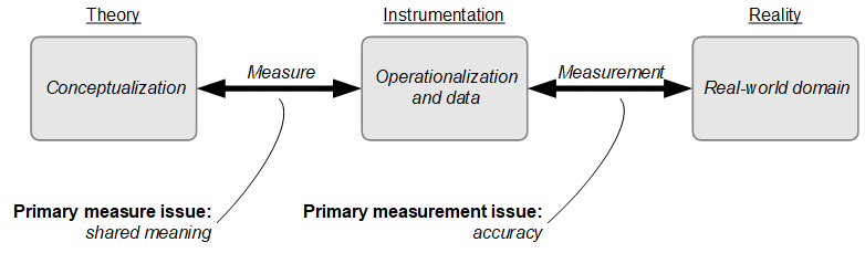
Understanding and addressing these challenges are important, independent from whether the research is about confirmation or exploration. In research concerned with confirmation, problems accumulate from the left to the right of Figure 2: If researchers fail to ensure shared meaning between their theoretical constructs and operationalizations, this restricts their ability to measure faithfully the constructs they theorized. In research concerned with exploration, problems tend to accumulate from the right to the left of Figure 2: No matter how well or systematically researchers explore their data, they cannot guarantee that their conclusions reflect reality unless they first take steps to ensure the accuracy of their data.
To avoid these problems, two key requirements must be met to avoid problems of shared meaning and accuracy and to ensure high quality of measurement:
- The variables that are chosen as operationalizations to measure a theoretical construct must share its meaning (in all its complexity if needed). This step concerns the validity of the measures.
- The variables that are chosen as operationalizations must also guarantee that data can be collected from the selected empirical referents accurately (i.e., consistently and precisely). This step concerns the reliability of measurement.
Together, validity and reliability are the benchmarks against which the adequacy and accuracy (and ultimately the quality) of QtPR are evaluated. To assist researchers, useful Respositories of measurement scales are available online. See for example: https://en.wikibooks.org/wiki/Handbook_of_Management_Scales.
4.2 Validity
Validity describes whether the operationalizations and the collected data share the true meaning of the constructs that the researchers set out to measure. Valid measures represent the essence or content upon which the construct is focused. For instance, recall the challenge of measuring “compassion”: A question of validity is to demonstrate that measurements are focusing on compassion and not on empathy or other related constructs.
There are different types of validity that are important to identify. Some of them relate to the issue of shared meaning and others to the issue of accuracy. In turn, there are theoretical assessments of validity (for example, for content validity,), which assess how well an operationalized measure fits the conceptual definition of the relevant theoretical construct; and empirical assessments of validity (for example, for convergent and discriminant validity), which assess how well collected measurements behave in relation to the theoretical expectations. Note that both theoretical and empirical assessments of validity are key to ensuring validity of study results.
Content validity in our understanding refers to the extent to which a researcher’s conceptualization of a construct is reflected in her operationalization of it, that is, how well a set of measures match with and capture the relevant content domain of a theoretical construct (Cronbach, 1971). But as with many other concepts, one should note that other characterizations of content validity also exist (e.g., Rossiter, 2011).
The key question of content validity in our understanding is whether the instrumentation (questionnaire items, for example) pulls in a representative manner all of the ways that could be used to measure the content of a given construct (Straub et al., 2004). Content validity is important because researchers have many choices in creating means of measuring a construct. Did they choose wisely so that the measures they use capture the essence of the construct? They could, of course, err on the side of inclusion or exclusion. If they include measures that do not represent the construct well, measurement error results. If they omit measures, the error is one of exclusion. Suppose you included “satisfaction with the IS staff” in your measurement of a construct called User Information Satisfaction but you forgot to include “satisfaction with the system” itself? Other researchers might feel that you did not draw well from all of the possible measures of the User Information Satisfaction construct. They could legitimately argue that your content validity was not the best. Assessments may include an expert panel that peruse a rating scheme and/or a qualitative assessment technique such as the Q-sort method (Block, 1961).
Construct validity is an issue of operationalization and measurement between constructs. With construct validity, we are interested in whether the instrumentation allows researchers to truly capture measurements for constructs in a way that is not subject to common methods bias and other forms of bias. For example, construct validity issues occur when some of the questionnaire items, the verbiage in the interview script, or the task descriptions in an experiment are ambiguous and are giving the participants the impression that they mean something different from what was intended.
Problems with construct validity occur in three major ways. Items or phrases in the instrumentation are not related in the way they should be, or they are related in the ways they should not be. If items do not converge, i.e., measurements collected with them behave statistically different from one another, it is called a convergent validity problem. If they do not segregate or differ from each other as they should, then it is called a discriminant validity problem.
Nomological validity assesses whether measurements and data about different constructs correlate in a way that matches how previous literature predicted the causal (or nomological) relationships of the underlying theoretical constructs. So, essentially, we are testing whether our obtained data fits previously established causal models of the phenomenon including prior suggested classifications of constructs (e.g., as independent, dependent, mediating, or moderating). If there are clear similarities, then the instrument items can be assumed to be reasonable, at least in terms of their nomological validity.
There are numerous ways to assess construct validity (Straub, Boudreau, and Gefen, 2004; Gefen, Straub, and Boudreau, 2000; Straub, 1989). Typically, researchers use statistical, correlational logic, that is, they attempt to establish empirically that items that are meant to measure the same constructs have similar scores (convergent validity) whilst also being dissimilar to scores of measures that are meant to measure other constructs (discriminant validity) This is usually done by comparing item correlations and looking for high correlations between items of one construct and low correlations between those items and items associated with other constructs. Other tests include factor analysis (a latent variable modeling approach) or principal component analysis (a composite-based analysis approach), both of which are tests to assess whether items load appropriately on constructs represented through a mathematically latent variable (a higher order factor). In this context, loading refers to the correlation coefficient between each measurement item and its latent factor. If items load appropriately high (viz., above 0.7), we assume that they reflect the theoretical constructs. Tests of nomological validity typically involve comparing relationships between constructs in a “network” of theoretical constructs with theoretical networks of constructs previously established in the literature and which may involve multiple antecedent, mediator, and outcome variables. The idea is to test a measurement model established given newly collected data against theoretically-derived constructs that have been measured with validated instruments and tested against a variety of persons, settings, times, and, in the case of IS research, technologies, in order to make the argument more compelling that the constructs themselves are valid (Straub et al. 2004). Often, such tests can be performed through structural equation modelling or moderated mediation models.
Internal validity assesses whether alternative explanations of the dependent variable(s) exist that need to be ruled out (Straub, 1989). It differs from construct validity, in that it focuses on alternative explanations of the strength of links between constructs whereas construct validity focuses on the measurement of individual constructs. Shadish et al. (2001) distinguish three factors of internal validity, these being (1) temporal precedence of IVs before DVs; (2) covariation; and (3) the ability to show the predictability of the current model variables over other, missing variables (“ruling out rival hypotheses”).
Challenges to internal validity in econometric and other QtPR studies are frequently raised using the rubric of “endogeneity concerns.” Endogeneity is an important issue because issues such as omitted variables, omitted selection, simultaneity, common-method variance, and measurement error all effectively render statistically estimates causally uninterpretable (Antonakis et al., 2010). Statistically, the endogeneity problem occurs when model variables are highly correlated with error terms. From a practical standpoint, this almost always happens when important variables are missing from the model. Hence, the challenge is what Shadish et al. (2001) are referring to in their third criterion: How can we show we have reasonable internal validity and that there are not key variables missing from our models?
Historically, internal validity was established through the use of statistical control variables. (Note that this is an entirely different concept from the term “control” used in an experiment where it means that one or more groups have not gotten an experimental treatment; to differentiate it from controls used to discount other explanations of the DV, we can call these “experimental controls.”) Statistical control variables are added to models to demonstrate that there is little-to-no explained variance associated with the designated statistical controls. Typical examples of statistical control variables in many QtPR IS studies are measurements of the size of firm, type of industry, type of product, previous experience of the respondents with systems, and so forth. Other endogeneity tests of note include the Durbin-Wu-Hausman (DWH) test and various alternative tests commonly carried out in econometric studies (Davidson and MacKinnon, 1993). If the DWH test indicates that there may be endogeneity, then the researchers can use what are called “instrumental variables” to see if there are indeed missing variables in the model. An overview of endogeneity concerns and ways to address endogeneity issues through methods such as fixed-effects panels, sample selection, instrumental variables, regression discontinuity, and difference-in-differences models, is given by Antonakis et al. (2010). More discussion on how to test endogeneity is available in Greene (2012).
Manipulation validity is used in experiments to assess whether an experimental group (but not the control group) is faithfully manipulated – and we can thus reasonably trust that any observed group differences are in fact attributable to the experimental manipulation. This form of validity is discussed in greater detail, including stats for assessing it, in Straub, Boudreau, and Gefen (2004). Suffice it to say at this point that in experiments, it is critical that the subjects are manipulated by the treatments and, conversely, that the control group is not manipulated. Checking for manipulation validity differs by the type and the focus of the experiment, and its manipulation and experimental setting. In some (nut not all) experimental studies, one way to check for manipulation validity is to ask subjects, provided they are capable of post-experimental introspection: Those who were aware that they were manipulated are testable subjects (rather than noise in the equations). In fact, those who were not aware, depending on the nature of the treatments, may be responding as if they were assigned to the control group.
In closing, we note that the literature also mentions other categories of validity. For example, statistical conclusion validity tests the inference that the dependent variable covaries with the independent variable, as well as that of any inferences regarding the degree of their covariation (Shadish et al., 2001). Type I and Type II errors are classic violations of statistical conclusion validity (Garcia-Pérez, 2012; Shadish et al., 2001). Predictive validity (Cronbach & Meehl, 1955) assesses the extent to which a measure successfully predicts a future outcome that is expected and practically meaningful. Finally, ecological validity (Shadish et al., 2001) assesses the ability to generalize study findings from an experimental setting to a set of real-world settings. High ecological validity means researchers can generalize the findings of their research study to real-life settings. We note that at other times, we have discussed ecological validity as a form of external validity (Im & Straub, 2015).
4.3 Reliability
Reliability describes the extent to which a measurement variable or set of variables is consistent in what it is intended to measure across multiple applications of measurements (e.g., repeated measurements or concurrently through alternative measures). If multiple measurements are taken, reliable measurements should all be consistent in their values.
Reliability is important to the scientific principle of replicability because reliability implies that the operations of a study can be repeated in equal settings with the same results. Consider the example of weighing a person. An unreliable way of measuring weight would be to ask onlookers to guess a person’s weight. Most likely, researchers will receive different answers from different persons (and perhaps even different answers from the same person if asked repeatedly). A more reliable way, therefore, would be to use a scale. Unless the person’s weight actually changes in the times between stepping repeatedly on to the scale, the scale should consistently, within measurement error, give you the same results. Note, however, that a mis-calibrated scale could still give consistent (but inaccurate) results. This example shows how reliability ensures consistency but not necessarily accuracy of measurement. Reliability does not guarantee validity.
Sources of reliability problems often stem from a reliance on overly subjective observations and data collections. All types of observations one can make as part of an empirical study inevitably carry subjective bias because we can only observe phenomena in the context of our own history, knowledge, presuppositions, and interpretations at that time. This is why often in QtPR researchers often look to replace observations made by the researcher or other subjects with other, presumably more “objective” data such as publicly verified performance metrics rather than subjectively experienced performance. Other sources of reliability problems stem from poorly specified measurements, such as survey questions that are imprecise or ambiguous, or questions asked of respondents who are either unqualified to answer, unfamiliar with, predisposed to a particular type of answer, or uncomfortable to answer.
Different types of reliability can be distinguished: Internal consistency (Streiner, 2003) is important when dealing with multidimensional constructs. It measures whether several measurement items that propose to measure the same general construct produce similar scores. The most common test is through Cronbach’s (1951) alpha, however, this test is not without problems. One problem with Cronbach alpha is that it assumes equal factor loadings, aka essential tau-equivalence. An alternative to Cronbach alpha that does not assume tau-equivalence is the omega test (Hayes and Coutts, 2020). The omega test has been made available in recent versions of SPSS; it is also available in other statistical software packages. Another problem with Cronbach’s alpha is that a higher alpha can most often be obtained simply by adding more construct items in that alpha is a function of k items. In other words, many of the items may not be highly interchangeable, highly correlated, reflective items (Jarvis et al., 2003), but this will not be obvious to researchers unless they examine the impact of removing items one-by-one from the construct.
Interrater reliability is important when several subjects, researchers, raters, or judges code the same data(Goodwin, 2001). Often, we approximate “objective” data through “inter-subjective” measures in which a range of individuals (multiple study subjects or multiple researchers, for example) all rate the same observation – and we look to get consistent, consensual results. Consider, for example, that you want to score student thesis submissions in terms of originality, rigor, and other criteria. We typically have multiple reviewers of such thesis to approximate an objective grade through inter-subjective rating until we reach an agreement. In scientific, quantitative research, we have several ways to assess interrater reliability. Cohen’s (1960) coefficient Kappa is the most commonly used test. Pearson’s or Spearman correlations, or percentage agreement scores are also used (Goodwin, 2001).
Straub, Boudreau, and Gefen (2004) introduce and discuss a range of additional types of reliability such as unidimensional reliability, composite reliability, split-half reliability, or test-retest reliability. They also list the different tests available to examine reliability in all its forms.
The demonstration of reliable measurements is a fundamental precondition to any QtPR study: Put very simply, the study results will not be trusted (and thus the conclusions foregone) if the measurements are not consistent and reliable. And because even the most careful wording of questions in a survey, or the reliance on non-subjective data in data collection does not guarantee that the measurements obtained will indeed be reliable, one precondition of QtPR is that instruments of measurement must always be tested for meeting accepted standards for reliability.
4.4 Developing and Assessing Measures and Measurements
Establishing reliability and validity of measures and measurement is a demanding and resource-intensive task. It is by no means “optional.” Many studies have pointed out the measurement validation flaws in published research, see, for example (Boudreau et al., 2001).
Because developing and assessing measures and measurement is time-consuming and challenging, researchers should first and always identify existing measures and measurements that have already been developed and assessed, to evaluate their potential for reuse. Aside from reducing effort and speeding up the research, the main reason for doing so is that using existing, validated measures ensures comparability of new results to reported results in the literature: analyses can be conducted to compare findings side-by-side. However, critical judgment is important in this process because not all published measurement instruments have in fact been thoroughly developed or validated; moreover, standards and knowledge about measurement instrument development and assessment themselves evolve with time. For example, several historically accepted ways to validate measurements (such as approaches based on average variance extracted, composite reliability, or goodness of fit indices) have later been criticized and eventually displaced by alternative approaches. As an example, Henseler et al. (2015) propose to evaluate heterotrait-monotrait correlation ratios instead of the traditional Fornell-Larcker criterion and the examination of cross-loadings when evaluating discriminant validity of measures.
There are great resources available that help researchers to identify reported and validated measures as well as measurements. For example, the Inter-Nomological Network (INN, https://inn.theorizeit.org/), developed by the Human Behavior Project at the Leeds School of Business, is a tool designed to help scholars to search the available literature for constructs and measurement variables (Larsen & Bong, 2016). Other management variables are listed on a wiki page.
When new measures or measurements need to be developed, the good news is that ample guidelines exist to help with this task. Historically, QtPR scholars in IS research often relied on methodologies for measurement instrument development that build on the work by Churchill in the field of marketing (Churchill, 1979). Figure 3 shows a simplified procedural model for use by QtPR researchers who wish to create new measurement instruments for conceptually defined theory constructs. The procedure shown describes a blend of guidelines available in the literature, most importantly (MacKenzie et al., 2011; Moore & Benbasat, 1991). It incorporates techniques to demonstrate and assess the content validity of measures as well as their reliability and validity. It separates the procedure into four main stages and describes the different tasks to be performed (grey rounded boxes), related inputs and outputs (white rectangles), and the relevant literature or sources of empirical data required to carry out the tasks (dark grey rectangles).
It is important to note that the procedural model as shown in Figure 3 describes this process as iterative and discrete, which is a simplified and idealized model of the actual process. In reality, any of the included stages may need to be performed multiple times and it may be necessary to revert to an earlier stage when the results of a later stage do not meet expectations. Also note that the procedural model in Figure 3 is not concerned with developing theory; rather it applies to the stage of the research where such theory exists and is sought to be empirically tested. In other words, the procedural model described below requires the existence of a well-defined theoretical domain and the existence of well-specified theoretical constructs.
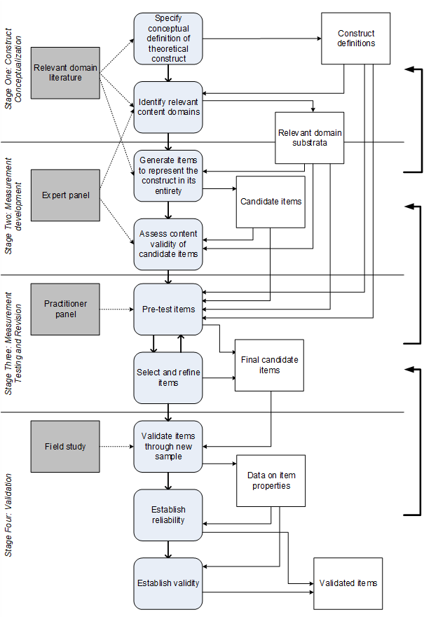
The first stage of the procedural model is construct conceptualization, which is concerned with defining the conceptual content domain of a construct. This task involves identifying and carefully defining what the construct is intended to conceptually represent or capture, discussing how the construct differs from other related constructs that may already exist, and defining any dimensions or domains that are relevant to grasping and clearly defining the conceptual theme or content of the construct it its entirety. MacKenzie et al. (2011) provide several recommendations for how to specify the content domain of a construct appropriately, including defining its domain, entity, and property.
A common problem at this stage is that researchers assume that labelling a construct with a name is equivalent to defining it and specifying its content domains: It is not. As a rule of thumb, each focal construct needs (1) a label, (2) a definition, (3) ideally one or more examples that demonstrate its meaning, and ideally (4) a discussion of related constructs in the literature, and (5) a discussion of the focal construct’s likely nomological net and its position within (e.g., as independent factor, as mediating or moderating factor, or as dependent factor).
The next stage is measurement development, where pools of candidate measurement items are generated for each construct. This task can be carried out through an analysis of the relevant literature or empirically by interviewing experts or conducting focus groups. This stage also involves assessing these candidate items, which is often carried out through expert panels that need to sort, rate, or rank items in relation to one or more content domains of the constructs. There are several good illustrations in the literature to exemplify how this works (e.g., Doll & Torkzadeh, 1998; MacKenzie et al., 2011; Moore & Benbasat, 1991).
The third stage, measurement testing and revision, is concerned with “purification”, and is often a repeated stage where the list of candidate items is iteratively narrowed down to a set of items that are fit for use. As part of that process, each item should be carefully refined to be as accurate and exact as possible. Often, this stage is carried out through pre- or pilot-tests of the measurements, with a sample that is representative of the target research population or else another panel of experts to generate the data needed. Repeating this stage is often important and required because when, for example, measurement items are removed, the entire set of measurement item changes, the result of the overall assessment may change, as well as the statistical properties of individual measurement items remaining in the set.
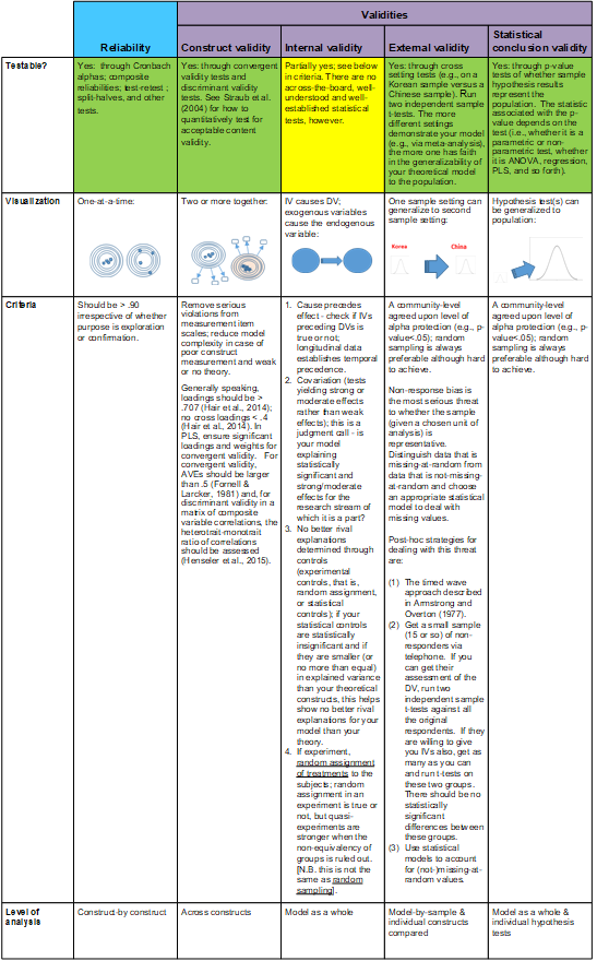
The final stage is validation, which is concerned with obtaining statistical evidence for reliability and validity of the measures and measurements. This task can be fulfilled by performing any field-study QtPR method (such as a survey or experiment) that provides a sufficiently large number of responses from the target population of the respective study. The key point to remember here is that for validation, a new sample of data is required – it should be different from the data used for developing the measurements, and it should be different from the data used to evaluate the hypotheses and theory. Figure 4 summarizes criteria and tests for assessing reliability and validity for measures and measurements. More details on measurement validation are discussed in Section 5 below.
Section 5: The General QtPR Research Approach
5.1 Defining the Purpose of a Study
Initially, a researcher must decide what the purpose of their specific study is: Is it confirmatory or is it exploratory research? Hair et al. (2010) suggest that confirmatory studies are those seeking to test (i.e., estimating and confirming) a prespecified relationship, whereas exploratory studies are those that define possible relationships in only the most general form and then allow multivariate techniques to search for non-zero or “significant” (practically or statistically) relationships. In the latter case, the researcher is not looking to “confirm” any relationships specified prior to the analysis, but instead allows the method and the data to “explore” and then define the nature of the relationships as manifested in the data.
5.2 Distinguishing Methods from Techniques
One of the most common issues in QtPR papers is mistaking data collection for method(s). When authors say their method was a survey, for example, they are telling the readers how they gathered the data, but they are not really telling what their method was. For example, their method could have been some form of an experiment that used a survey questionnaire to gather data before, during, or after the experiment. Or, the questionnaire could have been used in an entirely different method, such as a field study of users of some digital platform.
The same thing can be said about many econometric studies and other studies using archival data or digital trace data from an organization. Saying that the data came from an ecommerce platform or from scraping posts at a website is not a statement about method. It is simply a description of where the data came from.
Therefore, QtPR can involve different techniques for data collection and analysis, just as qualitative research can involve different techniques for data collection (such as focus groups, case study, or interviews) and data analysis (such as content analysis, discourse analysis, or network analysis).
To understand different types of QtPR methods, it is useful to consider how a researcher designs for variable control and randomization in the study. This allows comparing methods according to their validities (Stone, 1981). In this perspective, QtPR methods lie on a continuum from study designs where variables are merely observed but not controlled to study designs where variables are very closely controlled. Likewise, QtPR methods differ in the extent to which randomization is employed during data collection (e.g., during sampling or manipulations). Figure 5 uses these distinctions to introduce a continuum that differentiates four main types of general research approaches to QtPR.
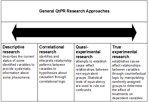
Within each type of QtPR research approach design, many choices are available for data collection and analysis. It should be noted that the choice of a type of QtPR research (e.g., descriptive or experimental) does not strictly “force” a particular data collection or analysis technique. It may, however, influence it, because different techniques for data collection or analysis are more or less well suited to allow or examine variable control; and likewise different techniques for data collection are often associated with different sampling approaches (e.g., non-random versus random). For example, using a survey instrument for data collection does not allow for the same type of control over independent variables as a lab or field experiment. Or, experiments often make it easier for QtPR researchers to use a random sampling strategy in comparison to a field survey. Similarly, the choice of data analysis can vary: For example, covariance structural equation modeling does not allow determining the cause-effect relationship between independent and dependent variables unless temporal precedence is included. Different approaches follow different logical traditions (e.g., correlational versus counterfactual versus configurational) for establishing causation (Antonakis et al., 2010; Morgan & Winship. 2015).
Typically, a researcher will decide for one (or multiple) data collection techniques while considering its overall appropriateness to their research, along with other practical factors, such as: desired and feasible sampling strategy, expected quality of the collected data, estimated costs, predicted nonresponse rates, expected level of measure errors, and length of the data collection period (Lyberg and Kasprzyk, 1991). It is, of course, possible that a given research question may not be satisfactorily studied because specific data collection techniques do not exist to collect the data needed to answer such a question (Kerlinger, 1986).
Popular data collection techniques for QtPR include: secondary data sources, observation, objective tests, interviews, experimental tasks, questionnaires and surveys, or q-sorting. These may be considered to be the instrumentation by which the researcher gathers data. Instrumentation in this sense is thus a collective term for all of the tools, procedures, and instruments that a researcher may use to gather data. Many of these data collection techniques require a research instrument, such as a questionnaire or an interview script. Others require coding, recoding, or transformation of the original data gathered through the collection technique.
The term “research instrument” can be preferable to specific names such as “survey instruments” in many situations. The term “research instrument” is neutral and does not imply a methodology. A research instrument can be administered as part of several different research approaches, e.g., as part of an experiment, a web survey, or a semi-structured interview.
Variable Control and Validity
Field studies tend to be high on external validity, but low on internal validity. Since the data is coming from the real world, the results can likely be generalized to other similar real-world settings. Hence the external validity of the study is high. On the other hand, field studies typically have difficulties controlling for the three internal validity factors (Shadish et al., 2001). Since field studies often involve statistical techniques for data analysis, the covariation criterion is usually satisfied. Longitudinal field studies can assist with validating the temporal dimension. But countering the possibility of other explanations for the phenomenon of interest is often difficult in most field studies, econometric studies being no exception.
At the other end of the continuum (Figure 6) we see approaches such as laboratory experimentation, which are commonly high on internal validity, but fairly low on external validity. Since laboratory experiments most often give one group a treatment (or manipulation) of some sort and another group no treatment, the effect on the DV has high internal validity. This is particularly powerful when the treatment is randomly assigned to the subjects forming each group. If they are randomly assigned, then there is a low probability that the effect is caused by any factors other than the treatment. Assuming that the experimental treatment is not about gender, for example, each group should be statistically similar in terms of its gender makeup. The same conclusion would hold if the experiment was not about preexisting knowledge of some phenomenon. Random assignment makes it highly unlikely that subjects’ prior knowledge impacted the DV. By their very nature, experiments have temporal precedence. The treatments always precede the collection of the DVs. Therefore, experimentation covers all three Shadish et al. (2001) criteria for internal validity.
Of special note is the case of field experiments. They involve manipulations in a real world setting of what the subjects experience. In the classic Hawthorne experiments, for example, one group received better lighting than another group. The experimental hypothesis was that the work group with better lighting would be more productive. The point here is not whether the results of this field experiment were interesting (they were, in fact, counter-intuitive). Rather, the point here is that internal validity is reasonably high in field experiments since they were conducted in real world settings. And since the results of field experiments are more generalizable to real-life settings than laboratory experiments (because they occur directly within real-life rather than artificial settings), they score also relatively high on external validity. One caveat in this case might be that the assignment of treatments in field experiments is often by branch, office, or division and there may be some systematic bias in choosing these sample frames in that it is not random assignment. All other things being equal, field experiments are the strongest method that a researcher can adopt.
Randomization
There are typically three forms of randomization employed in social science research methods. One form of randomization (random assignment) relates to the use of treatments or manipulations (in experiments, most often) and is therefore an aspect of internal validity (Trochim et al., 2016). Random assignment is about randomly manipulating the instrumentation so that there is a very unlikely connection between the group assignments (in an experimental block design) and the experimental outcomes. An example may help solidify this important point. The experimenter might use a random process to decide whether a given subject is in a treatment group or a control group. Thus the experimental instrumentation each subject experiences is quite different. Since the assignment to treatment or control is random, it effectively rules out almost any other possible explanation of the effect. Randomizing gender and health of participants, for example, should result in roughly equal splits between experimental groups so the likelihood of a systematic bias in the results from either of these variables is low. By chance, of course, there could be a preponderance of males or unhealthier persons in one group versus the other but in such rare cases researchers can regulate this in media res and adjust the sampling using a quota process (Trochim et al., 2016). Random assignment helps to establish the causal linkage between the theoretical antecedents and the effects and thereby strengthens internal validity.
A second form of randomization (random selection) relates to sampling, that is, the procedures used for taking a predetermined number of observations from a larger population, and is therefore an aspect of external validity (Trochim et al. 2016). Random selection is about choosing participating subjects at random from a population of interest. This is the surest way to be able to generalize from the sample to that population and thus a strong way to establish external validity. Another way to extend external validity within a research study is to randomly vary treatment levels. Again, an example might help explain this rarely used form of randomization. A researcher expects that the time it takes a web page to load (download delay in seconds) will adversely affect one’s patience in remaining at the website. The typical way to set treatment levels would be a very short delay, a moderate delay and a long delay. The issue is not whether the delay times are representative of the experience of many people. They may well be. But setting these exact points in the experiment means that we can generalize only to these three delay points. Randomizing the treatment times, however, allows a scholar to generalize across the whole range of delays, hence increasing external validity within the same, alternatively designed study.
A third form of randomization (random item inclusion) relates to how well a construct’s measures capture the content of a construct and is therefore an aspect of content validity (Straub et al. 2004). Random item inclusion means assuring content validity in a construct by drawing randomly from the universe of all possible measures of a given construct. Tests of content validity (e.g., through Q-sorting) are basically intended to verify this form of randomization. The fact of the matter is that the universe of all items is quite unknown and so we are groping in the dark to capture the best measures. They are truly socially-constructed.
Needless to say, this brief discussion only introduces three aspects to the role of randomization. There is a wealth of literature available to dig deeper into the role, and forms, of randomization (e.g., Cochran, 1977; Trochim et al., 2016; Shadish et al., 2001).
5.3 Descriptive and Correlational Research via Survey Instruments Collection
Descriptive and correlational research usually involves non-experimental, observational data collection techniques, such as survey instruments, which do not involve controlling or manipulating independent variables. This means that survey instruments in this research approach are used when one does not principally seek to intervene in reality (as in experiments), but merely wishes to observe it (even though the administration of a survey itself is already an intervention).
A survey is a means of gathering information about the characteristics, actions, perceptions, attitudes, or opinions of a large group of units of observations (such as individuals, groups or organizations), referred to as a population. Surveys thus involve collecting data about a large number of units of observation from a sample of subjects in field settings through questionnaire-type instruments that contain sets of printed or written questions with a choice of answers, and which can be distributed and completed via mail, online, telephone, or, less frequently, through structured interviewing. The resulting data is analyzed, typically through descriptive or inferential statistical techniques.
Surveys have historically been the dominant technique for data collection in information systems (Mazaheri et al. 2020). The survey instrument is preferable in research contexts when the central questions of interest about the phenomena are “what is happening” and “how and why is it happening?” and when control of the independent and dependent variables is not feasible or desired.
Research involving survey instruments in general can be used for at least three purposes, these being exploration, description, or explanation. The purpose of survey research in exploration is to become more familiar with a phenomenon or topic of interest. It focuses on eliciting important constructs and identifying ways for measuring these. Exploratory surveys may also be used to uncover and present new opportunities and dimensions about a population of interest. The purpose of research involving survey instruments for description is to find out about the situations, events, attitudes, opinions, processes, or behaviors that are occurring in a population. Thereby, descriptive surveys ascertain facts. They do not develop or test theory. The purpose of research involving survey instruments for explanation is to test theory and hypothetical causal relations between theoretical constructs. It is the most common form of survey instrument use in information systems research. Explanatory surveys ask about the relations between variables often on the basis of theoretically grounded expectations about how and why the variables ought to be related. Typically, the theory behind survey research involves some elements of cause and effect in that not only assumptions are made about relationships between variables but also about the directionality of these relationships. Surveys then allow obtaining correlations between observations that are assessed to evaluate whether the correlations fit with the expected cause and effect linkages. Surveys in this sense therefore approach causality from a correlational viewpoint; it is important to note that there are other traditions toward causal reasoning (such as configurational or counterfactual), some of which cannot be well-matched with data collected via survey research instruments (Antonakis et al., 2010; Pearl, 2009).
5.4 Experimental and Quasi-Experimental Research
Descriptive and correlational data collection techniques, such as surveys, rely on data sampling – the process of selecting units from a population of interest and observe or measure variables of interest without attempting to influence the responses. Such data, however, is often not perfectly suitable for gauging cause and effect relationships due to potential confounding factors that may exist beyond the data that is collected. And, crucially, inferring temporal precedence, i.e., establishing that the cause came before the effect, in a one-point in time survey is at best related to self-reporting by the subject.
Experiments are specifically intended to examine cause and effect relationships. This is because in experiments the researchers deliberately impose some treatment to one or more groups of respondents (the one or more treatment groups) but not to another group (the control group) while also maintaining control over other potential confounding factors in order to observe responses. A treatment is a manipulation of the real world that an experimenter administers to the subjects (also known as experimental units) so that the experimenter can observe a response. The treatment in an experiment is thus how an independent variable is operationalized. A typical way this is done is to divide the subjects into groups randomly where each group is “treated” differently so that the differences in these treatments result in differences in responses across these groups as hypothesize. Different treatments thus constitute different levels or values of the construct that is the independent variable.
The primary strength of experimental research over other research approaches is the emphasis on internal validity due to the availability of means to isolate, control and examine specific variables (the cause) and the consequence they cause in other variables (the effect). Its primary disadvantage is often a lack of ecological validity because the desire to isolate and control variables typically comes at the expense of realism of the setting. Moreover, real-world domains are often much more complex than the reduced set of variables that are being examined in an experiment.
Experimental research is often considered the gold standard in QtPR, but it is also one of the most difficult. This is because experimental research relies on very strong theory to guide construct definition, hypothesis specification, treatment design, and analysis. Any design error in experiments renders all results invalid. Moreover, experiments without strong theory tend to be ad hoc, possibly illogical, and meaningless because one essentially finds some mathematical connections between measures without being able to offer a justificatory mechanism for the connection (“you can’t tell me why you got these results”). The most pertinent danger in experiments is a flaw in the design that makes it impossible to rule out rival hypotheses (potential alternative theories that contradict the suggested theory). A second big problem is the inappropriate design of treatment and tasks.
Experiments can take place in the laboratory (lab experiments) or in reality (field experiments). Lab experiments typically offer the most control over the situation to the researcher, and they are the classical form of experiments. Think of students sitting in front of a computer in a lab performing experimental tasks or think of rats in cages that get exposed to all sorts of treatments under observation. Lauren Slater provides some wonderful examples in her book about experiments in psychology (Slater, 2005). Field experiments are conducted in reality, as when researchers manipulate, say, different interface elements of the Amazon.com webpage while people continue to use the ecommerce platform. Field experiments are difficult to set up and administer, in part because they typically involve collaborating with some organization that hosts a particular technology (say, an ecommerce platform). On the other hand, field experiments typically achieve much higher levels of ecological validity whilst also ensuring high levels of internal validity. They have become more popular (and more feasible) in information systems research over recent years.
In both lab and field experiments, the experimental design can vary (see Figures 6 and 7). For example, one key aspect in experiments is the choice of between-subject and within-subject designs: In between-subject designs, different people test each experimental condition. For example, if one had a treatment in the form of three different user-interface-designs for an e-commerce website, in a between-subject design three groups of people would each evaluate one of these designs. In a within-subjects design, the same subject would be exposed to all the experimental conditions. For example, each participant would first evaluate user-interface-design one, then the second user-interface-design, and then the third.
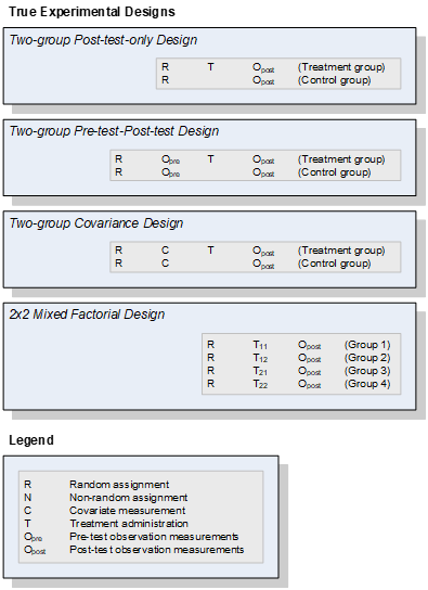
Quasi-experiments are similar to true experimental designs, with the difference being that they lack random assignment of subjects to groups, that is, experimental units are not assigned to experimental conditions randomly (Shadish et al., 2001). In effect, one group (say, the treatment group) may differ from another group in key characteristics; for example, a post-graduate class possesses higher levels of domain knowledge than an under-graduate class. Quasi-experimental designs often suffer from increased selection bias. Selection bias means that individuals, groups, or other data has been collected without achieving proper randomization, thereby failing to ensure that the sample obtained is representative of the population intended to be analyzed. Selection bias in turn diminishing internal validity. Still, sometimes a research design demands the deliberate assignment to an experimental group (for instance to explicitly test the effect of an intervention on under-performing students versus well-performing students). The most common forms are non-equivalent groups design – the alternative to a two-group pre-test-post-test design, and non-equivalent switched replication design, in which an essential experimental treatment is “replicated” by switching the treatment and control group in two subsequent iterations of the experiment (Trochim et al. 2016).
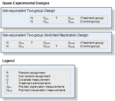
The literature also mentions natural experiments, which describe empirical studies in which subjects (or groups of subject) are exposed to different experimental and control conditions that are determined by nature or by other factors outside the control of the investigators (Dunning, 2012). Strictly speaking, natural experiments are not really experiments because the cause can usually not be manipulated; rather, natural experiments contrast naturally occurring events (e.g., an earthquake) with a comparison condition (Shadish et al., 2001). Free-simulation experiments (Tromkin & Steufert) expose subjects to real-world-like events and allow them within the controlled environment to behave generally freely and are asked to make decisions and choices as they see fit, thus allowing values of the independent variables to range over the natural range of the subjects’ experiences, and where ongoing events are determined by the interaction between experimenter-defined parameters (e.g., the prescribed experimental tasks) and the relatively free behavior of all participating subjects.
5.5 Quantitative Data Analysis
Data analysis concerns the examination of quantitative data in a number of ways. Descriptive analysis refers to describing, aggregating, and presenting the constructs of interests or the associations between the constructs to describe, for example, the population from where the data originated, the range of response levels obtained, and so forth. Inferential analysis refers to the statistical testing of hypotheses about populations based on a sample – typically the suspected cause and effect relationships – to ascertain whether the theory receives support from the data within certain degrees of confidence, typically described through significance levels. Most of these analyses are nowadays conducted through statistical software packages such as SPSS, SAS, or mathematical programming environments such as R or Mathematica. For any quantitative researcher, a good knowledge of these tools is essential.
There is not enough space here to cover the varieties or intricacies of different quantitative data analysis strategies. But many books exist on that topic (Bryman & Cramer, 2008; Field, 2013; Reinhart, 2015; Stevens, 2001; Tabachnick & Fidell, 2001), including one co-authored by one of us (Mertens et al., 2017).
Data analysis techniques include univariate analysis (such as analysis of single-variable distributions), bivariate analysis, and more generally, multivariate analysis. Univariate analyses concern the examination of one variable by itself, to identify properties such as frequency, distribution, dispersion, or central tendency. Classic statistics involve mean, median, variance, or standard deviation. Bivariate analyses concern the relationships between two variables. For example, we may examine the correlation between two numerical variables to identify the changes in one variable when the other variable levels increase or decrease. An example would be the correlation between salary increases and job satisfaction. A positive correlation would indicate that job satisfaction increases when pay levels go up. It is important to note here that correlation does not imply causation. A correlation between two variables merely confirms that the changes in variable levels behave in particular way upon changing another; but it cannot make a statement about which factor causes the change in variables (it is not unidirectional). Moreover, correlation analysis assumes a linear relationship. Should the relationship be other than linear, for example an inverted U relationship, then the results of a linear correlation analysis could be misleading. Multivariate analyses, broadly speaking, refer to all statistical methods that simultaneously analyze multiple measurements on each individual or object under investigation (Hair et al., 2010); as such, many multivariate techniques are extensions of univariate and bivariate analysis. The decision tree presented in Figure 8 provides a simplified guide for making the right choices.
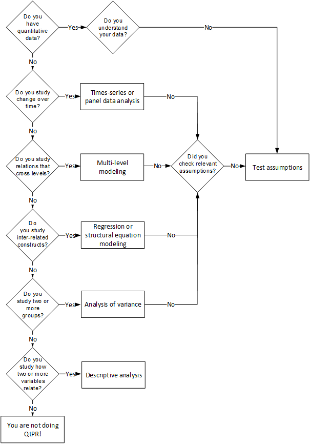
Figure 8 highlights that when selecting a data analysis technique, a researcher should make sure that the assumptions related to the technique are satisfied, such as normal distribution, independence among observations, linearity, and lack of multi-collinearity between the independent variables, and so forth (Mertens et al. 2017; Gefen, Straub, and Boudreau 2000; Gefen 2003). Multicollinearity can result in paths that are statistically significant when they should not be, they can be statistically insignificant when they are statistically significant, and they can even change the sign of a statistically significant path. Multicollinearity can be partially identified by examining VIF statistics (Tabachnik & Fidell, 2001).
The choice of the correct analysis technique is dependent on the chosen QtPR research design, the number of independent and dependent (and control) variables, the data coding and the distribution of the data received. This is because all statistical approaches to data analysis come with a set of assumptions and preconditions about the data to which they can be applied.
Most QtPR research involving survey data is analyzed using multivariate analysis methods, in particular structural equation modelling (SEM) through either covariance-based or component-based methods. Different methods in each tradition are available and are typically available in statistics software applications such as Stata, R, SPSS, or others. The most popular SEM methods include LISREL (Jöreskog & Sörbom, 2001) and equivalent software packages such as AMOS and Mplus, on the one hand, and Partial Least Squares (PLS) modeling (Chin, 2001; Hair et al., 2013), on the other hand.
SEM has been widely used in social science research for the causal modelling of complex, multivariate data sets in which the researcher gathers multiple measures of proposed constructs. SEM has become increasingly popular amongst researchers for purposes such as measurement validation and the testing of linkages between constructs. In general terms, SEM is a statistical method for testing and estimating assumed causal relationships using a combination of statistical data and qualitative causal assumptions. It encourages confirmatory rather than exploratory analysis. SEM requires one or more hypotheses between constructs, represented as a theoretical model, operationalizes by means of measurement items, and then tests statistically. The causal assumptions embedded in the model often have falsifiable implications that can be tested against survey data. One of the advantages of SEM is that many methods (such as covariance-based SEM models) cannot only be used to assess the structural model – the assumed causation amongst a set of multiple dependent and independent constructs – but also, separately or concurrently, the measurement model – the loadings of observed measurements on their expected latent constructs. In other words, SEM allows researchers to examine the reliability and validity of their measurements as well as the hypotheses contained in their proposed theoretical model. Several detailed step-by-step guides exist for running SEM analysis (e.g., Gefen, 2019; Ringle et al., 2012; Mertens et al., 2017; Henseler et al., 2015).
It should be noted at this point that other, different approaches to data analysis are constantly emerging. One of the most prominent current examples is certainly the set of Bayesian approaches to data analysis (Evermann & Tate, 2014; Gelman et al., 2013; Masson, 2011). Bayesian approaches are essentially model selection procedures that compute a comparison between competing hypotheses or models, and where available knowledge about parameters in a statistical model is updated with the information in observed data. The background knowledge is expressed as a prior distribution and combined with observational data in the form of a likelihood function to determine the posterior distribution. The posterior can also be used for making predictions about future events.
Most experimental and quasi-experimental studies use some form of between-groups analysis of variance such as ANOVA, repeated measures, or MANCOVA. An introduction is provided by Mertens et al. (2017). Standard readings on this matter are Shadish et al. (2001) and Trochim et al. (2016).
If the data or phenomenon concerns changes over time, an analysis technique is required that allows modeling differences in data over time. Essentially, time series data is single variable data that has another dimension of time. For example, the price of a certain stock over days weeks, months, quarters, or years. The most important difference between such time-series data and cross-sectional data is that the added time dimension of time-series data means that such variables change across both units and time. In other words, data can differ across individuals (a “between-variation”) at the same point in time but also internally across time (a “within-variation”).
To analyze data with a time dimension, several analytical tools are available that can be used to model how a current observation can be estimated by previous observations, or to forecast future observations based on that pattern. The difficulty in such analyses is to account for how events unfolding over time can be separated from the momentum of the past itself. For example, one way to analyze time-series data is by means of the Auto-Regressive Integrated Moving Average (ARIMA) technique, that captures how previous observations in a data series determine the current observation. It can also include other covariates. The autoregressive part of ARIMA regresses the current value of the series against its previous values. This can be the most immediate previous observation (a lag of order 1), a seasonal effect (such as the value this month last year, a lag of order 12), or any other combination of previous observations. The moving average part adds a linear combination of the error terms of the previous observations. The number of such previous error terms determines the order of the moving average. The integrated part of the model is included when there is a trend in the data, such as an increase over time, in which case the difference between the observations is calculated rather than modeling the actual observed values. This is necessary because if there is a trend in the series then the model cannot be stationary. Stationarity means that the mean and variance remain the same throughout the range of the series. A sample application of ARIMA in IS research is modeling the usage levels of a health information environments over time and how quasi-experimental events related to governmental policy changed it (Gefen et al., 2019). Other popular ways to analyze time-series data are latent variable models such as latent growth curve models, latent change score models, or bivariate latent difference score models (Bollen & Curran, 2006; McArdle, 2009).
5.6 Validation of Measures and Measurement
Recall that measurement is, arguably, the most important thing that a QtPR scholar can do to ensure that the results of their study can be trusted. Figure 9 shows how to prioritize the assessment of measurement during data analysis.
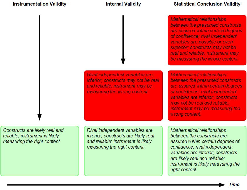
[Legend: green indicates preferred path; red indicates problematic path]
Row 1: Good statistical conclusion validity, poor internal validity
Imagine a situation where you carry out a series of statistical tests and find terrific indications for statistical significance. You are hopeful that your model is accurate and that the statistical conclusions will show that the relationships you posit are true and important.
Unfortunately, unbeknownst to you, the model you specify is wrong (in the sense that the model may omit common antecedents to both the independent and the dependent variables, or that it exhibits endogeneity concerns). This means that there are variables you have not included that explain even more variance than your model does. An example situation could be a structural equation model that supports the existence of some speculated hypotheses but also shows poor fit to the data. In such a situation you are in the worst possible scenario: you have poor internal validity but good statistical conclusion validity.
Row 2: Good internal validity, good statistical conclusion validity, poor instrumentation validity
Internal validity is a matter of causality. Can you rule out other reasons for why the independent and dependent variables in your study are or are not related? Consider the following: You are testing constructs to see which variable would or could “confound” your contention that a certain variable is as good an explanation for a set of effects. But statistical conclusion and internal validity are not sufficient, instrumentation validity (in terms of measurement validity and reliability) matter as well: Unreliable measurement leads to attenuation of regression path coefficients, i.e. the estimated effect size, whereas invalid measurement means you’re not measuring what you wanted to measure. So if either the posited independent variable or the confound (a rival variable) is poorly measured, then you cannot know with any certainty whether one or the other variable is the true cause. In this situation you have an internal validity problem that is really not simply a matter of testing the strength of either the confound or the theoretical independent variable on the outcome variable, but it is a matter of whether you can trust the measurement of either the independent, the confounding, or the outcome variable. Without instrumentation validity, it is really not possible to assess internal validity. In the early days of computing there was an acronym for this basic idea: GIGO. It stood for “garbage in, garbage out.” It meant that if the data being used for a computer program were of poor, unacceptable quality, then the output report was just as deficient. With respect to instrument validity, if one’s measures are questionable, then there is no data analysis technique that can fix the problem. Research results are totally in doubt if the instrument does not measure the theoretical constructs at a scientifically acceptable level.
Row 3: The only acceptable path (All forms of validity)
Assessing measure and measurement validity is the critical first step in QtPR. If your instrumentation is not acceptable at a minimal level, then the findings from the study will be perfectly meaningless. You cannot trust or contend that you have internal validity or statistical conclusion validity. Reviewers should be especially honed in to measurement problems for this reason. If the measures are not valid and reliable, then we cannot trust that there is scientific value to the work. In an experiment, for example, it is critical that a researcher check not only the experimental instrument, but also whether the manipulation or treatment works as intended, whether experimental task are properly phrased, and so forth.
Straub, Gefen, and Boudreau (2004) describe the “ins” and “outs” for assessing instrumentation validity. Their paper presents the arguments for why various forms of instrumentation validity should be mandatory and why others are optional. Basically, there are four types of scientific validity with respect to instrumentation. They are: (1) content validity, (2) construct validity, (3) reliability, and (4) manipulation validity (see also Figure 4).
Section 6. Practical Tips for Writing QtPR Papers
QtPR papers are welcomed in every information systems journal as QtPR is the most frequently used general research approach in information systems research both historically and currently (Vessey et al., 2020; Mazaheri et al., 2020). Many great examples exist as templates that can guide the writing of QtPR papers. In what follows, we give a few selected tips related to the crafting of such papers.
6.1 Developing Theory in QtPR Papers: Conceptual Labeling of Constructs
Constructs are socially constructed. That is to say, they are created in the mind as abstractions. Like the theoretical research model of construct relationships itself, they are intended to capture the essence of a phenomenon and then to reduce it to a parsimonious form that can be operationalized through measurements.
That being said, constructs are much less clear in what they represent when researchers think of them as entity-relationship (ER) models. ER models are highly useful for normalizing data, but do not serve well for social science research models. Why not? Entities themselves do not express well what values might lie behind the labeling. And in quantitative constructs and models, the whole idea is (1) to make the model understandable to others and (2) to be able to test it against empirical data. So communication of the nature of the abstractions is critical.
An example might help to explain this. Sometimes one sees a model when one of the constructs is “Firm.” It is unclear what this could possibly mean. Does it mean that the firm exists or not? Likely this is not the intention. On the other hand, “Size of Firm” is more easily interpretable, and this construct frequently appears, as noted elsewhere in this treatise. It implies that there will be some form of a quantitative representation of the presence of the firm in the marketplace.
As a second example, models in articles will sometimes have a grab-all variable/construct such as “Environmental Factors.” The problem here is similar to the example above. What could this possibly mean? Likely not that there are either environmental factors or not. The conceptual labeling of this construct is too broad to easily convey its meaning. Were it broken down into its components, there would be less room for criticism. One common construct in the category of “environmental factors,” for instance, is market uncertainty. As a conceptual labeling, this is superior in that one can readily conceive of a relatively quiet marketplace where risks were, on the whole, low. The other end of the uncertainty continuum can be envisioned as a turbulent marketplace where risk was high and economic conditions were volatile. And it is possible using the many forms of scaling available to associate this construct with market uncertainty falling between these end points.
A third example is construct labeling that could be clarified by simply adding a modifying word or phrase to show the reader more precisely what the construct means. Let’s take the construct labelled originally “Co-creation.” Again, the label itself is confusing (albeit typical) in that it likely does not mean that one is co-creating something or not. A clarifying phrase like “Extent of Co-creation” (as opposed to, say, “duration of co-creation”) helps interested readers in conceptualizing that there needs to be some kind of quantification of the amount but not length of co-creating taking place. The theory base itself will provide boundary conditions so that we can see that we are talking about a theory of how systems are designed (i.e., a co-creative process between users and developers) and how successful these systems then are. But the effective labelling of the construct itself can go a long way toward making theoretical models more intuitively appealing.
6.2 Should Dos, Could Dos, and Must Not Dos for QtPR Papers
The table in Figure 10 presents a number of guidelines for IS scholars constructing and reporting QtPR research based on, and extended from, Mertens and Recker (2020). The guidelines consist of three sets of recommendations: two to encourage (“should do” and “could do”) and one to discourage (“must not do”) practices. This combination of “should, could and must not do” forms a balanced checklist that can help IS researchers throughout all stages of the research cycle to protect themselves against cognitive biases (e.g., by preregistering protocols or hypotheses), improve statistical mastery where possible (e.g., through consulting independent methodological advice), and become modest, humble, contextualized, and transparent (Wasserstein et al., 2019) wherever possible (e.g., by following open science reporting guidelines and cross-checking terminology and argumentation).
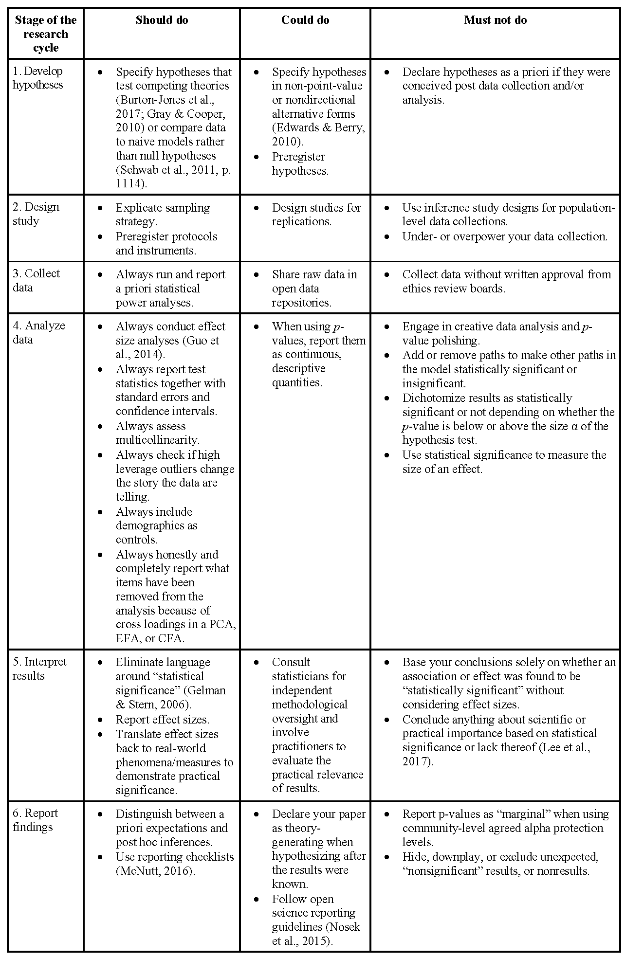
6.3 Using Personal Pronouns in QtPR Writing
When preparing a manuscript for either a conference or a journal submission, it can be advisable to use the personal pronouns “I” and “we” as little as possible. Of course, such usage of personal pronouns occurs in academic writing, but what it implies might distract from the main storyline of a QtPR article. The emphasis in sentences using the personal pronouns is on the researcher and not the research itself. “I did this, then I did that. Then I did something else.” Or “we did this, followed by our doing that. Next we did the other thing…” Such sentences stress the actions and activities of the researcher(s) rather than the purposes of these actions. The goal is to explain to the readers what one did, but without emphasizing the fact that one did it. The whole point is justifying what was done, not who did it. Converting active voice [this is what it is called when the subject of the sentence highlights the “actor(s)”] to passive voice is a trivial exercise. In a sentence structured in the passive voice, a different verbal form is used, such as in this very sentence. Sentences can also be transformed from active voice that utilizes the personal pronoun in many other ways. The easiest way to show this, perhaps, is through an example. Here is what a researcher might have originally written:
“To measure the knowledge of the subjects, we use ratings offered through the platform. In fact, there are several ratings that we can glean from the platform and these we will combine to create an aggregate score. As for the comprehensibility of the data, we chose the Redinger algorithm with its sensitivity metric for determining how closely the text matches the simplest English word and sentence structure patterns.”
To transform this same passage into passive voice is fairly straight-forward (of course, there are also many other ways to make sentences interesting without using personal pronouns):
“To measure the knowledge of the subjects, ratings offered through the platform were used. In fact, several ratings readily gleaned from the platform were combined to create an aggregate score. As for the comprehensibility of the data, the best choice is the Redinger algorithm with its sensitivity metric for determining how closely the text matches the simplest English word and sentence structure patterns.”
As a caveat, note that many researchers prefer the use of personal pronouns in their writings to emphasize the fact that they are interpreting data through their own personal lenses and that conclusions may not be generalizable. Avoiding personal pronouns can likewise be a way to emphasize that QtPR scientists were deliberately trying to “stand back” from the object of the study.
Section 7: Glossary
Adaptive experiment:
This is a “quasi-experimental” research methodology that involves before and after measures, a control group, and non-random assignment of human subjects. Data are gathered before the independent variables are introduced, but the final form is not usually known until after the independent variables have been introduced and the “after” data has been collected (Jenkins, 1985).
Archival research:
This methodology is primarily concerned with the examination of historical documents. Secondarily, it is concerned with any recorded data. All data are examined ex-post-facto by the researcher (Jenkins, 1985).
ANOVA:
Univariate analysis of variance (ANOVA) is a statistical technique to determine, on the basis of one dependent measure, whether samples come from populations with equal means. ANOVA is fortunately robust to violations of equal variances across groups (Lindman, 1974). Univariate analysis of variance employs one dependent measure, whereas multivariate analysis of variance compares samples based on two or more dependent variables.
ANCOVA:
Analysis of covariance (ANCOVA) is a form of analysis of variance that tests the significance of the differences among means of experimental groups after taking into account initial differences among the groups and the correlation of the initial measures and the dependent variable measures. The measure used as a control variable – the pretest or pertinent variable – is called a covariate (Kerlinger, 1986). Covariates need to be at least interval data and will help to partial out the variance and strengthen main effects.
Canonical correlation:
With canonical analysis the objective is to correlate simultaneously several metric dependent variables and several metric independent variables. The underlying principle is to develop a linear combination of each set of variables (both independent and dependent) to maximize the correlation between the two sets.
Cluster analysis:
Cluster analysis is an analytical technique for developing meaningful sub-groups of individuals or objects. Specifically, the objective is to classify a sample of entities (individuals or objects) into a smaller number of mutually exclusive groups based on the similarities among the entities (Hair et al., 2010).
Content domain:
The content domain of an abstract theoretical construct specifies the nature of that construct and its conceptual theme in unambiguous terms and as clear and concise as possible (MacKenzie et al., 2011). The content domain of a construct should formally specify the nature of the construct, including the conceptual domain to which the focal construct belongs and the entity to which it applies.
Conjoint analysis:
Conjoint analysis is an emerging dependence technique that has brought new sophistication to the evaluation of objects, whether they are new products, services, or ideas. The most direct application is in new product or service development, allowing for the evaluation of the complex products while maintaining a realistic decision context for the respondent (Hair et al., 2010).
Correspondence analysis:
Correspondence analysis is a recently developed interdependence technique that facilitates both dimensional reduction of object ratings (e.g., products, persons, etc.) on a set of attributes and the perceptual mapping of objects relative to these attributes (Hair et al., 2010).
Dependent variable:
A variable whose value is affected by, or responds to, a change in the value of some independent variable(s).
Experimental simulation:
This methodology employs a closed simulation model to mirror a segment of the “real world.” Human subjects are exposed to this model and their responses are recorded. Thee researcher completely determines the nature and timing of the experimental events (Jenkins, 1985).
Factor analysis:
Factor analysis is a statistical approach that can be used to analyze interrelationships among a large number of variables and to explain these variables in terms of their common underlying dimensions (factors) (Hair et al., 2010).
Field experiments:
Field experiments involve the experimental manipulation of one or more variables within a naturally occurring system and subsequent measurement of the impact of the manipulation on one or more dependent variables (Boudreau et al., 2001).
Field studies:
Field studies are non-experimental inquiries occurring in natural systems. Researchers using field studies typically do not manipulate independent variables or control the influence of confounding variables (Boudreau et al., 2001).
Free simulation experiment:
This methodology is similar to experimental simulation, in that with both methodologies the researcher designs a closed setting to mirror the “real world” and measures the response of human subjects as they interact within the system. However, with this methodology, events and their timing are determined by both the researcher and the behavior of the human subject (Jenkins, 1985; Fromkin and Streufert, 1976).
Hotelling’s T2:
A test statistic to assess the statistical significance of the difference between two sets of sample means. It is a special case of MANOVA used with two groups or levels of a treatment variable (Hair et al., 2010).
Independent Variable:
A variable whose value change is presumed to cause a change in the value of some dependent variable(s).
Lab(oratory) experiments:
Laboratory experiments take place in a setting especially created by the researcher for the investigation of the phenomenon. With this research method, the researcher has control over the independent variable(s) and the random assignment of research participants to various treatment and non-treatment conditions (Boudreau et al., 2001).
Linear probability models:
In this technique, one or more independent variables are used to predict a single dependent variable. Linear probability models accommodate all types of independent variables (metric and non-metric) and do not require the assumption of multivariate normality (Hair et al., 2010).
Linear regression:
A linear regression attempts determine the best equation describing a set of x and y data points, by using an optimization function such as least squares or maximum likelihood.
LISREL:
A procedure for the analysis of LInear Structural RELations among one or more sets of variables and variates. It examines the covariance structures of the variables and variates included in the model under consideration. LISREL permits both confirmatory factor analysis and the analysis of path models with multiple sets of data in a simultaneous analysis.
Loading (Factor Loading):
A weighting that reflects the correlation between the original variables and derived factors. Squared factor loadings are the percent of variance in an observed item that is explained by its factor.
LOGIT:
Logit analysis is a special form of regression in which the criterion variable is a non-metric, dichotomous (binary) variable. While differences exist in some aspects, the general manner of interpretation is quite similar to linear regression (Hair et al., 2010).
Math modeling:
This methodology models the “real world” and states the results as mathematical equations. It is a closed deterministic system in which all of the independent and dependent variables are known and included in the model. Intervening variables simply are not possible and no human subject is required (Jenkins, 1985).
MTMM:
Multitrait-multimethod (MTMM) uses a matrix of correlations representing all possible relationships between a set of constructs, each measured by the same set of methods. This matrix is one of many methods that can be used to evaluate construct validity by demonstrating both convergent and discriminant validity.
Multidimensional scaling:
In multidimensional scaling, the objective is to transform consumer judgments of similarity or preference (e.g., preference for stores or brands) into distances in a multidimensional space. If objects A and B are judged by respondents as being the most similar compared with all other possible pairs of objects, multidimensional scaling techniques will position objects A and B in such a way that the distance between them in the multidimensional space is smaller than the distance between any other two pairs of objects. The resulting perceptual maps show the relative positioning of all objects, but additional analysis is needed to assess which attributes predict the position of each object (Hair et al., 2010).
Multiple regression:
Multiple regression is the appropriate method of analysis when the research problem involves a single metric dependent variable presumed to be related to one or more metric independent variables. The objective of multiple regression analysis is to predict the changes in the dependent variable in response to the changes in the several independent variables (Hair et al., 2010).
Multiple discriminant analysis:
If the single dependent variable is dichotomous (e.g., male-female) or multichotomous (e.g., high-medium-low) and therefore non-metric, the multivariate technique of multiple discriminant analysis (MDA) is appropriate. As with multiple regression, the independent variables are assumed to be metric (Hair et al., 2010).
Multivariate analysis of variance (MANOVA):
Multivariate analysis of variance (MANOVA) is a statistical technique that can be used to simultaneously explore the relationship between several categorical independent variables (usually referred to as treatments) and two or more metric dependent variables. As such, it represents an extension of univariate analysis of variance (ANOVA). MANOVA is useful when the researcher designs an experimental situation (manipulation of several non-metric treatment variables) to test hypotheses concerning the variance in group responses on two or more metric dependent variables (Hair et al., 2010).
Normal Distribution:
A normal distribution is probably the most important type of distribution in behavioral sciences and is the underlying assumption of many of the statistical techniques discussed here. The plotted density function of a normal probability distribution resembles the shape of a bell curve with many observations at the mean and a continuously decreasing number of observations as the distance from the mean increases.
Multinormal distribution:
Also known as a Joint Normal Distribution and as a Multivariate Normal Distribution, occurs when every polynomial combination of items itself has a Normal Distribution. For example, in Linear Regression the dependent variable Y may be the polynomial combination of aX1+bX2+e, where it is assumed that X1 and X2 each has a normal distribution. Multinormal distribution occurs when also the polynomial expression aX1+bX2 itself has a normal distribution. Graphically, a multinormal distribution of X1 and X2 will resemble a sheet of paper with a weight at its center, the center being analogous to the mean of the joint distribution.
Objective Tests:
A type of assessment instrument consisting of a set of items or questions that have specific correct answers (e.g., how much is 2 + 2?), such that no interpretation, judgment, or personal impressions are involved in scoring.
Observation:
Observation means looking at people and listening to them talk. One can infer the meaning, characteristics, motivations, feelings and intentions of others on the basis of observations (Kerlinger, 1986).
PLS (Partial Least Squares) path modeling:
A second generation regression component-based estimation approach that combines a composite analysis with linear regression. .Unlike covariance-based approaches to structural equation modeling, PLS path modeling does not fit a common factor model to the data, it rather fits a composite model.
PCA: Principal Components Analysis.
A dimensionality-reduction method that is often used to transform a large set of variables into a smaller one of uncorrelated or orthogonal new variables (known as the principal components) that still contains most of the information in the large set. Principal components are new variables that are constructed as linear combinations or mixtures of the initial variables such that the principal components account for the largest possible variance in the data set. The objective is to find a way of condensing the information contained in a number of original variables into a smaller set of principal component variables with a minimum loss of information (Hair et al., 2010).
Q-sorting:
Q-sorting offers a powerful, theoretically grounded, and quantitative tool for examining opinions and attitudes. Q-sorting consists of a modified rank-ordering procedure in which stimuli are placed in an order that is significant from the standpoint of a person operating under specified conditions. It results in the captured patterns of respondents to the stimulus presented, a topic on which opinions vary. Those patterns can then be analyzed to discover groupings of response patterns, supporting effective inductive reasoning (Thomas and Watson, 2002).
Reliability:
Extent to which a variable or set of variables is consistent in what it measures. If multiple (e.g., repeated) measurements are taken, the reliable measures will all be very consistent in their values.
R-squared or R2: Coefficient of determination:
Measure of the proportion of the variance of the dependent variable about its mean that is explained by the independent variable(s). R-squared is derived from the F statistic. This statistic is usually employed in linear regression analysis and PLS. In LISREL, the equivalent statistic is known as a squared multiple correlation.
Secondary data sources:
Data that was already collected for some other purpose is called secondary data. Organization files and library holdings are the most frequently used secondary sources of data. Statistical compendia, movie film, printed literature, audio tapes, and computer files are also widely used sources. Secondary data sources can be usually found quickly and cheaply. Sometimes there is no alternative to secondary sources, for example, census reports and industry statistics. Secondary data also extend the time and space range, for example, collection of past data or data about foreign countries (Emory, 1980).
SEM (Structural Equation Modeling):
A label for a variety of multivariate statistical techniques that can include confirmatory factor analysis, confirmatory composite analysis, path analysis, multi-group modeling, longitudinal modeling, partial least squares path modeling, latent growth modeling and hierarchical or multi-level modeling. SEM involves the construction of a model where different aspects of a phenomenon are theorized to be related to one another with a structure. This structure is a system of equations that captures the statistical properties implied by the model and its structural features, and which is then estimated with statistical algorithms (usually based on matrix algebra and generalized linear models) using experimental or observational data.
Time-series analysis:
A data analysis technique used to identify how a current observation is estimated by previous observations, or to predict future observations based on that pattern. Time-series analysis can be run as an Auto-Regressive Integrated Moving Average (ARIMA) model that specifies how previous observations in the series determine the current observation. It can include also cross-correlations with other covariates. Other techniques include OLS fixed effects and random effects models (Mertens et al., 2017).
Wilks’ Lambda: One of the four principal statistics for testing the null hypothesis in MANOVA. It is also referred to as the maximum likelihood criterion or U statistic (Hair et al., 2010).
Section 8: Bibliography
8.1 Further Readings
There is a large variety of excellent resources available to learn more about QtPR. You can learn more about the philosophical basis of QtPR in writings by Karl Popper (1959) and Carl Hempel (1965). Introductions to their ideas and those of relevant others are provided by philosophy of science textbooks (e.g., Chalmers, 1999; Godfrey-Smith, 2003). There are also articles on how information systems builds on these ideas, or not (e.g., Siponen & Klaavuniemi, 2020).
If you are interested in different procedural models for developing and assessing measures and measurements, you can read up on the following examples that report at some lengths about their development procedures: (Bailey & Pearson, 1983; Davis, 1989; Goodhue, 1998; Moore & Benbasat, 1991; Recker & Rosemann, 2010; Bagozzi, 2011).
Textbooks on survey research that are worth reading include Floyd Flower’s textbook (Fowler, 2001), Devellis and Thorpe (2021), plus a few others (Babbie, 1990; Czaja & Blair, 1996). It is also important to regularly check for methodological advances in journal articles, such as (Baruch & Holtom, 2008; Kaplowitz et al., 2004; King & He, 2005).
A seminal book on experimental research has been written by William Shadish, Thomas Cook, and Donald Campbell (Shadish et al., 2001). A wonderful introduction to behavioral experimentation is Lauren Slater’s book Opening Skinner’s Box: Great Psychological Experiments of the Twentieth Century (Slater, 2005).
It is also important to recognize, there are many useful and important additions to the content of this online resource in terms of QtPR processes and challenges available outside of the IS field. For example, the computer sciences also have an extensive tradition in discussing QtPR notions, such as threats to validity. Wohlin et al.’s (2000) book on Experimental Software Engineering, for example, illustrates, exemplifies, and discusses many of the most important threats to validity, such as lack of representativeness of independent variable, pre-test sensitisation to treatments, fatigue and learning effects, or lack of sensitivity of dependent variables. Vegas and colleagues (2016) discuss advantages and disadvantages between a wide range of experiment designs, such as independent measures, repeated measures, crossover, matched-pairs, and different mixed designs.
Another important debate in the QtPR realm is the ongoing discussion on reflective versus formative measurement development, which was not covered in this resource. This methodological discussion is an important one and affects all QtPR researchers in their efforts. Several viewpoints pertaining to this debate are available (Aguirre-Urreta & Marakas, 2012; Centefelli & Bassellier, 2009; Diamantopoulos, 2001; Diamantopoulos & Siguaw, 2006; Diamantopoulos & Winklhofer, 2001; Kim et al., 2010; Petter et al., 2007).
Another debate in QtPR is about the choice of analysis approaches and toolsets. For example, there is a longstanding debate about the relative merits and limitations of different approaches to structural equation modelling (Goodhue et al., 2007, 2012; Hair et al., 2011; Marcoulides & Saunders, 2006; Ringle et al., 2012), including alternative approaches such as Bayesian structural equation modeling (Evermann & Tate, 2014), or the TETRAD approach (Im & Wang, 2007). These debates, amongst others, also produce several updates to available guidelines for their application (e.g., Henseler et al., 2014; Henseler et al., 2015; Rönkkö & Cho, 2022).
Another debate concerns alternative models for reasoning about causality (Pearl, 2009; Antonakis et al., 2010; Bollen & Pearl, 2013) based on a growing recognition that causality itself is a socially constructed term and many statistical approaches to testing causality are imbued with one particular philosophical perspective toward causality.
Finally, there is debate about the future of hypothesis testing (Branch, 2014; Cohen, 1994; Pernet, 2016; Schwab et al., 2011; Szucs & Ioannidis, 2017; Wasserstein & Lazar, 2016; Wasserstein et al., 2019). This debate focuses on the existence, and mitigation, of problematic practices in the interpretation and use of statistics that involve the well-known p-value. One aspect of this debate focuses on supplementing p-value testing with additional analysis that extra the meaning of the effects of statistically significant results (Lin et al., 2013; Mohajeri et al., 2020; Sen et al., 2022). These proposals essentially suggest retaining p-values. Alternative proposals essentially focus on abandoning the notion that generalizing to the population is the key concern in hypothesis testing (Guo et al., 2014; Kline, 2013) and instead moving from generalizability to explanatory power, for example, by relying on correlations to determine what effect sizes are reasonable in different research settings.
There is a large variety of excellent resources available to learn more about QtPR. You can learn more about the philosophical basis of QtPR in writings by Karl Popper (1959) and Carl Hempel (1965). Introductions to their ideas and those of relevant others are provided by philosophy of science textbooks (e.g., Chalmers, 1999; Godfrey-Smith, 2003). There are also articles on how information systems builds on these ideas, or not (e.g., Siponen & Klaavuniemi, 2020).
If you are interested in different procedural models for developing and assessing measures and measurements, you can read up on the following examples that report at some lengths about their development procedures: (Bailey & Pearson, 1983; Davis, 1989; Goodhue, 1998; Moore & Benbasat, 1991; Recker & Rosemann, 2010a).
Textbooks on survey research that are worth reading include Floyd Flower’s textbook (Fowler, 2001) plus a few others (Babbie, 1990; Czaja & Blair, 1996). It is also important to regularly check for methodological advances in journal articles, such as (Baruch & Holtom, 2008; Kaplowitz et al., 2004; King & He, 2005).
A seminal book on experimental research has been written by William Shadish, Thomas Cook, and Donald Campbell (Shadish et al., 2001). A wonderful introduction to behavioral experimentation is Lauren Slater’s book “Opening Skinner’s Box: Great Psychological Experiments of the Twentieth Century” (Slater, 2005).
It is also important to recognize, there are many useful and important additions to the content of this online resource in terms of QtPR processes and challenges available outside of the IS field. For example, the computer sciences also have an extensive tradition in discussing QtPR notions, such as threats to validity. Claes Wohlin’s book on Experimental Software Engineering (Wohlin et al., 2000), for example, illustrates, exemplifies, and discusses many of the most important threats to validity, such as lack of representativeness of independent variable, pre-test sensitisation to treatments, fatigue and learning effects, or lack of sensitivity of dependent variables. Sira Vegas and colleagues (Vegas et al., 2016) discuss advantages and disadvantages between a wide range of experiment designs, such as independent measures, repeated measures, crossover, matched-pairs, and different mixed designs.
Another important debate in the QtPR realm is the ongoing discussion on reflective versus formative measurement development. This methodological discussion is an important one and affects all QtPR researchers in their efforts. Several viewpoints pertaining to this debate are available (Aguirre-Urreta & Marakas, 2012; Centefelli & Bassellier, 2009; Diamantopoulos, 2001; Diamantopoulos & Siguaw, 2006; Diamantopoulos & Winklhofer, 2001; Kim et al., 2010; Petter et al., 2007).
Another debate in QtPR is about the choice of analysis approaches and toolsets. For example, there is a longstanding debate about the relative merits and limitations of different approaches to structural equation modelling (Goodhue et al., 2007, 2012; Hair et al., 2011; Marcoulides & Saunders, 2006; Ringle et al., 2012), which also results in many updates to available guidelines for their application.
Finally, there is a perennial debate in QtPR about null hypothesis significance testing (Branch, 2014; Cohen, 1994; Pernet, 2016; Schwab et al., 2011; Szucs & Ioannidis, 2017; Wasserstein & Lazar, 2016; Wasserstein et al., 2019). This debate focuses on the existence, and mitigation, of problematic practices in the interpretation and use of statistics that involve the well-known p value. We have co-authored a set of updated guidelines for quantitative researchers for dealing with these issues (Mertens & Recker, 2020).
8.2 References
Aguirre-Urreta, M. I., & Marakas, G. M. (2012). Revisiting Bias Due to Construct Misspecification: Different Results from Considering Coefficients in Standardized Form. MIS Quarterly, 36(1), 123-138.
Antonakis, J., Bendahan, S., Jacquart, P., & Lalive, R. (2010). On Making Causal Claims: A Review and Recommendations. The Leadership Quarterly, 21(6), 1086-1120.
Babbie, E. R. (1990). Survey Research Methods. Wadsworth.
Bagozzi, R.P. (1980), Causal Methods in Marketing. John Wiley and Sons.
Bagozzi, R. P. (2011). Measurement and Meaning in Information Systems and Organizational Research: Methodological and Philosophical Foundations. MIS Quarterly, 35(2), 261-292.
Bailey, J. E., & Pearson, S. W. (1983). Development of a Tool for Measuring and Analyzing Computer User Satisfaction. Management Science, 29(5), 530-545.
Baruch, Y., & Holtom, B. C. (2008). Survey Response Rate Levels and Trends in Organizational Research. Human Relations, 61(8), 1139-1160.
Block, J. (1961). The Q-Sort Method in Personality Assessment and Psychiatric Research. Charles C Thomas Publisher.
Bollen, K. A. (1989) Structural Equations with Latent Variables. New York: John Wiley and Sons.
Bollen, K. A., & Curran, P. J. (2006). Latent Curve Models: A Structural Equation Perspective. John Wiley & Sons.
Boudreau, M.-C., Gefen, D., & Straub, D. W. (2001). Validation in Information Systems Research: A State-of-the-Art Assessment. MIS Quarterly, 25(1), 1-16.
Branch, M. (2014). Malignant Side Effects of Null-hypothesis Significance Testing. Theory & Psychology, 24(2), 256-277.
Bryman, A., & Cramer, D. (2008). Quantitative Data Analysis with SPSS 14, 15 & 16: A Guide for Social Scientists. Routledge.
Burton-Jones, A., & Lee, A. S. (2017). Thinking About Measures and Measurement in Positivist Research: A Proposal for Refocusing on Fundamentals. Information Systems Research, 28(3), 451-467.
Burton-Jones, A., Recker, J., Indulska, M., Green, P., & Weber, R. (2017). Assessing Representation Theory with a Framework for Pursuing Success and Failure. MIS Quarterly, 41(4), 1307-1333.
Campbell, D.T., and Fiske, D.W. “Convergent and Discriminant Validation by the Multitrait- Multimethod Matrix,” Psychological Bulletin (56:2, March) 1959, pp 81-105.
Centefelli, R. T., & Bassellier, G. (2009). Interpretation of Formative Measurement in Information Systems Research. MIS Quarterly, 33(4), 689-708.
Chalmers, A. F. (1999). What Is This Thing Called Science? (3rd ed.). Hackett.
Chin, W. W. (2001). PLS-Graph user’s guide. CT Bauer College of Business, University of Houston, USA, 15, 1-16.
Christensen, R. (2005). Testing Fisher, Neyman, Pearson, and Bayes. The American Statistician, 59(2), 121-126.
Churchill Jr., G. A. (1979). A Paradigm for Developing Better Measures of Marketing Constructs. Journal of Marketing Research, 16(1), 64-73.
Clark, P. A. (1972). Action Research and Organizational Change. Harper and Row.
Cochran, W. G. (1977). Sampling Techniques (3rd ed.). John Wiley & Sons.
Cohen, J. (1960). A Coefficient of Agreement for Nominal Scales. Educational and Psychological Measurement, 20(1), 37-46.
Cohen, J. (1988). Statistical Power Analysis for the Behavioral Sciences (2nd ed.). Lawrence Erlbaum Associates.
Cohen, J. (1994). The Earth is Round (p < .05). American Psychologist, 49(12), 997-1003.
Cook, T. D. and D. T. Campbell (1979). Quasi Experimentation: Design and Analytical Issues for Field Settings. Chicago, Rand McNally.
Coombs, C. H. (1976). A Theory of Data. Mathesis Press.
Corder, G. W., & Foreman, D. I. (2014). Nonparametric Statistics for Non-Statisticians: A Step-by-Step Approach (2nd ed.). Wiley.
Cronbach, L. J., & Meehl, P. E. (1955). Construct Validity in Psychological Tests. Psychological Bulletin, 52(4), 281-302.
Cronbach, L. J. (1951). Coefficient Alpha and the Internal Structure of Tests. Psychometrika, 16(3), 291-334.
Cronbach, L. J. (1971). Test Validation. In R. L. Thorndike (Ed.), Educational Measurement (2nd ed., pp. 443-507). American Council on Education.
Czaja, R. F., & Blair, J. (1996). Designing Surveys: A Guide to Decisions and Procedures. Pine Forge Press.
Davidson, R., & MacKinnon, J. G. (1993). Estimation and Inference in Econometrics. Oxford University Press.
Davis, F. D. (1989). Perceived Usefulness, Perceived Ease of Use, and User Acceptance of Information Technology. MIS Quarterly, 13(3), 319-340.
DeVellis, R. F., & Thorpe, C. T. (2021). Scale Development: Theory and Applications (5th ed.). Sage.
Diamantopoulos, A. (2001). Incorporating Formative Measures into Covariance-Based Structural Equation Models. MIS Quarterly, 35(2), 335-358.
Diamantopoulos, A., & Siguaw, J. A. (2006). Formative Versus Reflective Indicators in Organizational Measure Development: A Comparison and Empirical Illustration. British Journal of Management, 17(4), 263-282.
Diamantopoulos, Adamantios and Heidi M. Winklhofer, “Index Construction with Formative Indicators: An Alternative to Scale Development,” Journal of Marketing Research, 38, 2, (2001), 269-277.
Doll, W. J., & Torkzadeh, G. (1988). The Measurement of End-User Computing Satisfaction. MIS Quarterly, 12(2), 259-274.
Dunning, T. (2012). Natural Experiments in the Social Sciences: A Design-Based Approach. Cambridge University Press.
Edwards, J. R., & Berry, J. W. (2010). The Presence of Something or the Absence of Nothing: Increasing Theoretical Precision in Management Research. Organizational Research Methods, 13(4), 668-689.
Elden, M., & Chisholm, R. F. (1993). Emerging Varieties of Action Research: Introduction to the Special Issue. Human Relations, 46(2), 121-142.
Emory, W. C. (1980). Business Research Methods. Irwin.
Evermann, J., & Tate, M. (2011). Fitting Covariance Models for Theory Generation. Journal of the Association for Information Systems, 12(9), 632-661.
Evermann, J., & Tate, M. (2014). Bayesian Structural Equation Models for Cumulative Theory Building in Information Systems―A Brief Tutorial Using BUGS and R. Communications of the Association for Information Systems, 34(77), 1481-1514.
Falk, R., & Greenbaum, C. W. (1995). Significance Tests Die Hard: The Amazing Persistence of a Probabilistic Misconception. Theory & Psychology, 5(1), 75-98.
Field, A. (2013). Discovering Statistics using IBM SPSS Statistics. Sage.
Fisher, R. A. (1935). The Logic of Inductive Inference. Journal of the Royal Statistical Society, 98(1), 39-82.
Fisher, R. A. (1935). The Design of Experiments. Oliver and Boyd.
Fisher, R. A. (1955). Statistical Methods and Scientific Induction. Journal of the Royal Statistical Society. Series B (Methodological), 17(1), 69-78.
Fornell, C., & Larcker, D. F. (1981). Evaluating Structural Equations with Unobservable Variables and Measurement Error. Journal of Marketing Research, 18(1), 39-50.
Fowler, F. J. (2001). Survey Research Methods (3rd ed.). Sage.
Fromkin, H. L., & Streufert, S. (1976). Laboratory Experimentation. Rand McNally College Publishing Company.
Garcia-Pérez, M. A. (2012). Statistical Conclusion Validity: Some Common Threats and Simple Remedies. Frontiers in Psychology, 3(325), 1-11.
Gasson, S. (2004). Rigor in Grounded Theory Research: An Interpretive Perspective on Generating Theory from Qualitative Field Studies. In M. E. Whitman & A. B. Woszczynski (Eds.), The Handbook of Information Systems Research (pp. 79-102). Idea Group Publishing.
Gefen, D., Ben-Assuli, O., Stehr, M., Rosen, B., & Denekamp, Y. (2019). Governmental Intervention in Hospital Information Exchange (HIE) Diffusion: A Quasi-Experimental Arima Interrupted Time Series Analysis of Monthly HIE Patient Penetration Rates. European Journal of Information Systems, 17(5), 627-645.
Gefen, D., Straub, D. W., & Boudreau, M.-C. (2000). Structural Equation Modeling and Regression: Guidelines for Research Practice. Communications of the Association for Information Systems, 4(7), 1-77.
Gefen, D. (2003). Assessing Unidimensionality Through LISREL: An Explanation and an Example. Communications of the Association for Information Systems, 12(2), 23-47.
Gefen, D., & Larsen, K. R. T. (2017). Controlling for Lexical Closeness in Survey Research: A Demonstration on the Technology Acceptance Model. Journal of the Association for Information Systems, 18(10), 727-757.
Gefen, D. (2019). A Post-Positivist Answering Back. Part 2: A Demo in R of the Importance of Enabling Replication in PLS and LISREL. ACM SIGMIS Database, 50(3), 12-37.
Gelman, A. (2013). P Values and Statistical Practice. Epidemiology, 24(1), 69-72.
Gelman, A., Carlin, J. B., Stern, H., Dunson, D. B., Vehtari, A., & Rubin, D. B. (2013). Bayesian Data Analysis (3rd ed.). Chapman and Hall/CRC.
Gelman, A., & Stern, H. (2006). The Difference Between “Significant” and “Not Significant” is not Itself Statistically Significant. The American Statistician, 60(4), 328-331.
Gigerenzer, G. (2004). Mindless Statistics. Journal of Socio-Economics, 33(5), 587-606.
Glaser, B. G., & Strauss, A. L. (1967). The Discovery of Grounded Theory: Strategies for Qualitative Research. Aldine Publishing Company.
Godfrey-Smith, P. (2003). Theory and Reality: An Introduction to the Philosophy of Science. University of Chicago Press.
Goodhue, D. L. (1998). Development And Measurement Validity Of A Task-Technology Fit Instrument For User Evaluations Of Information Systems. Decision Sciences, 29(1), 105-139.
Goodhue, D. L., Lewis, W., & Thompson, R. L. (2007). Statistical Power in Analyzing Interaction Effects: Questioning the Advantage of PLS With Product Indicators. Information Systems Research, 18(2), 211-227.
Goodhue, D. L., Lewis, W., & Thompson, R. L. (2012). Comparing PLS to Regression and LISREL: A Response to Marcoulides, Chin, and Saunders. MIS Quarterly, 36(3), 703-716.
Goodwin, L. D. (2001). Interrater Agreement and Reliability. Measurement in Physical Education and Exercise Science, 5(1), 13-34.
Gray, P. H., & Cooper, W. H. (2010). Pursuing Failure. Organizational Research Methods, 13(4), 620-643.
Greene, W. H. (2012). Econometric Analysis (7th ed.). Pearson.
Greenland, S., Senn, S. J., Rothman, K. J., Carlin, J. B., Poole, C., Goodman, S. N., & Altman, D. G. (2016). Statistical Tests, P Values, Confidence Intervals, and Power: a Guide to Misinterpretations. European Journal of Epidemiology, 31(4), 337-350.
Gregor, S. (2006). The Nature of Theory in Information Systems. MIS Quarterly, 30(3), 611-642.
Guo, W., Straub, D. W., & Zhang, P. (2014). A Sea Change in Statistics: A Reconsideration of What Is Important in the Age of Big Data. Journal of Management Analytics, 1(4), 241-248.
Hair, J. F., Black, W. C., Babin, B. J., & Anderson, R. E. (2010). Multivariate Data Analysis (7th ed.). Prentice Hall.
Hair, J. F., Ringle, C. M., & Sarstedt, M. (2011). PLS-SEM: Indeed a Silver Bullet. The Journal of Marketing Theory and Practice, 19(2), 139-152.
Hair, J. F., Hult, G. T. M., Ringle, C. M., & Sarstedt, M. (2013). A Primer on Partial Least Squares Structural Equation Modeling (PLS-SEM). Sage.
Haller, H., & Kraus, S. (2002). Misinterpretations of Significance: A Problem Students Share with Their Teachers? Methods of Psychological Research, 7(1), 1-20.
Hayesa, A. F. and Coutts, J. J. (2020). Use Omega Rather than Cronbach’s Alpha for Estimating Reliability. But… Communication Methods and Measures (14,1), 1-24.
Hedges, L. V., & Olkin, I. (1985). Statistical Methods for Meta-Analysis. Academic Press.
Heisenberg, W. (1927). Über den anschaulichen Inhalt der quantentheoretischen Kinematik und Mechanik (in German). Zeitschrift für Physik, 43(3-4), 172-198.
Hempel, C. G. (1965). Aspects of Scientific Explanation and other Essays in the Philosophy of Science. The Free Press.
Henseler, J., Dijkstra, T. K., Sarstedt, M., Ringle, C. M., Diamantopoulos, A., Straub, D. W., Ketchen, D. J., Hair, J. F., Hult, G. T. M., & Calantone, R. J. (2014). Common Beliefs and Reality About PLS: Comments on Rönkkö and Evermann (2013). Organizational Research Methods, 17(2), 182-209.
Henseler, J., Ringle, C. M., & Sarstedt, M. (2015). A new Criterion for Assessing Discriminant Validity in Variance-based Structural Equation Modeling. Journal of the Academy of Marketing Science, 43(1), 115-135.
Im, G., & Straub, D. W. (2015). The Critical Role of External Validity in Organizational Theorizing. Communications of the Association for Information Systems, 37(44), 911-964.
Im, G., & Wang, J. (2007). A TETRAD-based Approach for Theory Development in Information Systems Research. Communications of the Association for Information Systems, 20(22), 322-345.
Jarvis, C. B., MacKenzie, S. B., & Podsakoff, P. M. (2003). A Critical Review of Construct Indicators and Measurement Model Misspecification in Marketing and Consumer Research. Journal of Consumer Research, 30(2), 199-218.
Jöreskog, K. G., & Sörbom, D. (2001). LISREL 8: User’s Reference Guide. Scientific Software International.
Kaplowitz, M. D., Hadlock, T. D., & Levine, R. (2004). A Comparison of Web and Mail Survey Response Rates. Public Opinion Quarterly, 68(1), 84-101.
Kim, G., Shin, B., & Grover, V. (2010). Investigating Two Contradictory Views of Formative Measurement in Information Systems Research. MIS Quarterly, 34(2), 345-366.
King, W. R., & He, J. (2005). External Validity in IS Survey Research. Communications of the Association for Information Systems, 16(45), 880-894.
Kline, R. B. (2013). Beyond Significance Testing: Statistics Reform in the Behavioral Sciences (2nd ed.). American Psychological Association.
Jenkins, A. M. (1985). Research Methodologies and MIS Research. In E. Mumford, R. Hirschheim, & A. T. Wood-Harper (Eds.), Research Methods in Information Systems (pp. 103-117). North-Holland.
Judd, C. M., Smith, E. R., & Kidder, L. H. (1991). Research Methods in Social Relations (6th ed.). Harcourt Brace College Publishers.
Kaplan, B., and Duchon, D. “Combining Qualitative and Quantitative Methods in Information Systems Research: A Case Study,” MIS Quarterly (12:4 (December)) 1988, pp. 571-586.
Kerlinger, F. N. (1986), Foundations of Behavioral Research, Harcourt Brace Jovanovich.
Lakatos, I. (1970). Falsification and the Methodology of Scientific Research Programs. In I. Lakatos & A. Musgrave (Eds.), Criticism and the Growth of Knowledge (pp. 91-132). Cambridge University Press.
Larsen, K. R. T., & Bong, C. H. (2016). A Tool for Addressing Construct Identity in Literature Reviews and Meta-Analyses. MIS Quarterly, 40(3), 529-551.
Lee, A. S., & Hubona, G. S. (2009). A Scientific Basis for Rigor in Information Systems Research. MIS Quarterly, 33(2), 237-262.
Lee, A. S., Mohajeri, K., & Hubona, G. S. (2017). Three Roles for Statistical Significance and the Validity Frontier in Theory Testing. 50th Hawaii International Conference on System Sciences, Waikoloa Village, Hawaii.
Lehmann, E. L. (1993). The Fisher, Neyman-Pearson Theories of Testing Hypotheses: One Theory or Two? Journal of the American Statistical Association, 88(424), 1242-1249.
Levallet, N., Denford, J. S., & Chan, Y. E. (2021). Following the MAP (Methods, Approaches, Perspectives) in Information Systems Research. Information Systems Research, 32(1), 130–146.
Lin, M., Lucas Jr., H. C., & Shmueli, G. (2013). Too Big to Fail: Large Samples and the p-Value Problem. Information Systems Research, 24(4), 906-917.
Lindman, H. R. (1974). ANOVA in Complex Experimental Designs. W. H. Freeman.
Lyberg, L. E., & Kasprzyk, D. (1991). Data Collection Methods and Measurement Error: An Overview. In P. P. Biemer, R. M. Groves, L. E. Lyberg, N. A. Mathiowetz, & S. Sudman (Eds.), Measurement Errors in Surveys (pp. 235-257). Wiley.
MacKenzie, S. B., Podsakoff, P. M., & Podsakoff, N. P. (2011). Construct Measurement and Validation Procedures in MIS and Behavioral Research: Integrating New and Existing Techniques. MIS Quarterly, 35(2), 293-334.
Marcoulides, G. A., & Saunders, C. (2006). Editor’s Comments: PLS: A Silver Bullet? MIS Quarterly, 30(2), iii-ix.
Masson, M. E. (2011). A Tutorial on a Practical Bayesian Alternative to Null-Hypothesis Significance Testing. Behavior Research Methods, 43(3), 679-690.
Mazaheri, E., Lagzian, M., & Hemmat, Z. (2020). Research Directions in Information Systems Field, Current Status and Future Trends: A Literature Analysis of AIS Basket of Top Journals. Australasian Journal of Information Systems, 24, doi:10.3127/ajis.v24i0.2045.
McArdle, J. J. (2009). Latent Variable Modeling of Differences and Changes with Longitudinal Data. Annual Review of Psychology, 60, 577-605.
McNutt, M. (2016). Taking Up TOP. Science, 352(6290), 1147.
McShane, B. B., & Gal, D. (2017). Blinding Us to the Obvious? The Effect of Statistical Training on the Evaluation of Evidence. Management Science, 62(6), 1707-1718.
Meehl, P. E. (1967). Theory-Testing in Psychology and Physics: A Methodological Paradox. Philosophy of Science, 34(2), 103-115.
Mertens, W., Pugliese, A., & Recker, J. (2017). Quantitative Data Analysis: A Companion for Accounting and Information Systems Research. Springer.
Mertens, W., & Recker, J. (2020). New Guidelines for Null Hypothesis Significance Testing in Hypothetico-Deductive IS Research. Journal of the Association for Information Systems, 21(4), 1072-1102.
Miller, J. (2009). What is the Probability of Replicating a Statistically Significant Effect? Psychonomic Bulletin & Review, 16(4), 617-640.
Miller, I., & Miller, M. (2012). John E. Freund’s Mathematical Statistics With Applications (8th ed.). Pearson Education.
Mohajeri, K., Mesgari, M., & Lee, A. S. (2020). When Statistical Significance Is Not Enough: Investigating Relevance, Practical Significance and Statistical Significance. MIS Quarterly, 44(2), 525-559.
Moore, G. C., & Benbasat, I. (1991). Development of an Instrument to Measure the Perceptions of Adopting an Information Technology Innovation. Information Systems Research, 2(3), 192-222.
Morgan, S. L., & Winship, C. (2014). Counterfactuals and Causal Inference: Methods and Principles for Social Research (2nd ed.). Cambridge University Press.
Myers, M. D. (2009). Qualitative Research in Business and Management. Sage.
Neyman, J., & Pearson, E. S. (1928). On the Use and Interpretation of Certain Test Criteria for Purposes of Statistical Inference: Part I. Biometrika, 20A(1/2), 175-240.
Neyman, J., & Pearson, E. S. (1933). On the Problem of the Most Efficient Tests of Statistical Hypotheses. Philosophical Transactions of the Royal Society of London. Series A, Containing Papers of a Mathematical or Physical Character, 231, 289-337.
Nosek, B. A., Alter, G., Banks, G. C., Borsboom, D., Bowman, S. D., Breckler, S. J., Buck, S., Chambers, C. D., Chin, G., Christensen, G., Contestabile, M., Dafoe, A., Eich, E., Freese, J., Glennerster, R., Goroff, D., Green, D. P., Hesse, B., Humphreys, M., Ishiyama, J., Karlan, D., Kraut, A., Lupia, A., Mabry, P., Madon, T., Malhotra, N., Mayo-Wilson, E., McNutt, M., Miguel, E., Paluck, E. L., Simonsohn, U., Soderberg, C., Spellman, B. A., Turitto, J., VandenBos, G., Vazire, S., Wagenmakers, E.-J., Wilson, R. L., & Yarkoni, T. (2015). Promoting an Open Research Culture. Science, 348(6242), 1422-1425.
Orne, M. T. (1962). On The Social Psychology of the Psychological Experiment: With Particular Reference to Demand Characteristics and their Implications. American Psychologist, 17(11), 776-783.
Pearl, J. (2009). Causality: Models, Reasoning, and Inference (2nd ed.). Cambridge University Press.
Pernet, C. (2016). Null Hypothesis Significance Testing: a Guide to Commonly Misunderstood Concepts and Recommendations for Good Practice [version 5; peer review: 2 approved, 2 not approved]. F1000Research, 4(621).
Petter, S., Straub, D. W., & Rai, A. (2007). Specifying Formative Constructs in IS Research. MIS Quarterly, 31(4), 623-656.
Popper, K. R. (1959). The Logic of Scientific Discovery. Basic Books. (Logik der Forschung, Vienna, 1935)
Recker, J. (2021). Scientific Research in Information Systems: A Beginner’s Guide (2nd ed.). Springer.
Recker, J., & Rosemann, M. (2010). A Measurement Instrument for Process Modeling Research: Development, Test and Procedural Model. Scandinavian Journal of Information Systems, 22(2), 3-30.
Reinhart, A. (2015). Statistics Done Wrong: The Woefully Complete Guide. No Starch Press.
Ringle, C. M., Sarstedt, M., & Straub, D. W. (2012). Editor’s Comments: A Critical Look at the Use of PLS-SEM in MIS Quarterly. MIS Quarterly, 36(1), iii-xiv.
Rönkkö, M., & Cho, E. (2022). An Updated Guideline for Assessing Discriminant Validity. Organizational Research Methods, 25(1), 6-14.
Rossiter, J. R. (2011). Measurement for the Social Sciences: The C-OAR-SE Method and Why It Must Replace Psychometrics. Springer.
Sarker, S., Xiao, X., Beaulieu, T., & Lee, A. S. (2018). Learning from First-Generation Qualitative Approaches in the IS Discipline: An Evolutionary View and Some Implications for Authors and Evaluators (PART 1/2). Journal of the Association for Information Systems, 19(8), 752-774.
Schwab, A., Abrahamson, E., Starbuck, W. H., & Fidler, F. (2011). PERSPECTIVE—Researchers Should Make Thoughtful Assessments Instead of Null-Hypothesis Significance Tests. Organization Science, 22(4), 1105-1120.
Sen, A., Smith, G., & Van Note, C. (2022). Statistical Significance Versus Practical Importance in Information Systems Research. Journal of Information Technology, 37(3), 288–300.
Shadish, W. R., Cook, T. D., & Campbell, D. T. (2001). Experimental and Quasi-Experimental Designs for Generalized Causal Inference (2nd ed.). Houghton Mifflin.
Siponen, M. T., & Klaavuniemi, T. (2020). Why is the Hypothetico-Deductive (H-D) Method in Information Systems not an H-D Method? Information and Organization, 30(1), 100287.
Slater, L. (2005). Opening Skinner’s Box: Great Psychological Experiments of the Twentieth Century. Norton & Company.
Stevens, J. P. (2001). Applied Multivariate Statistics for the Social Sciences (4th ed.). Lawrence Erlbaum Associates.
Stone, Eugene F., Research Methods in Organizational Behavior, Glenview, IL, 1981.
Straub, D. W., Gefen, D., & Boudreau, M.-C. (2005). Quantitative Research. In D. Avison & J. Pries-Heje (Eds.), Research in Information Systems: A Handbook for Research Supervisors and Their Students (pp. 221-238). Elsevier.
Straub, D. W., Boudreau, M.-C., & Gefen, D. (2004). Validation Guidelines for IS Positivist Research. Communications of the Association for Information Systems, 13(24), 380-427.
Straub, D. W. (1989). Validating Instruments in MIS Research. MIS Quarterly, 13(2), 147-169.
Streiner, D. L. (2003). Starting at the Beginning: An Introduction to Coefficient Alpha and Internal Consistency. Journal of Personality Assessment, 80(1), 99-103.
Szucs, D., & Ioannidis, J. P. A. (2017). When Null Hypothesis Significance Testing Is Unsuitable for Research: A Reassessment. Frontiers in Human Neuroscience, 11(390), 1-21.
Tabachnick, B. G., & Fidell, L. S. (2001). Using Multivariate Statistics (4th ed.). Allyn & Bacon.
Thomas, D. M., & Watson, R. T. (2002). Q-Sorting and MIS Research: A Primer. Communications of the Association for Information Systems, 8(9), 141-156.
Trochim, W. M. K., Donnelly, J. P., & Arora, K. (2016). Research Methods: The Essential Knowledge Base (2nd ed.). Cengage Learning.
Vegas, S., Apa, C., & Juristo, N. (2016). Crossover Designs in Software Engineering Experiments: Benefits and Perils. IEEE Transactions on Software Engineering, 42(2), 120-135.
Vessey, I., Ramesh, V., & Glass, R. L. (2002). Research in Information Systems: An Empirical Study of Diversity in the Discipline and Its Journals. Journal of Management Information Systems, 19(2), 129-174.
Walsham, G. (1995). Interpretive Case Studies in IS Research: Nature and Method. European Journal of Information Systems, 4, 74-81.
Wasserstein, R. L., & Lazar, N. A. (2016). The ASA’s Statement on P-values: Context, Process, and Purpose. The American Statistician, 70(2), 129-133.
Wasserstein, R. L., Schirm, A. L., & Lazar, N. A. (2019). Moving to a World Beyond “p < 0.05.” The American Statistician, 73(sup1), 1-19.
Wohlin, C., Runeson, P., Höst, M., Ohlsson, M. C., Regnell, B., & Wesslén, A. (2000). Experimentation in Software Engineering: An Introduction. Kluwer Academic Publishers.
Yin, R. K. (2009). Case Study Research: Design and Methods (4th ed.). Sage Publications.